Gantt chart

Check list
- 1) preparation
- 1.1) Familiarization with develop tools
- 1.1.1) Keras
- 1.1.2) Pythrch
- 1.2) Presentation
- 1.2.1) Poster conference
- 2) Create image database
- 2.1) Confirmation of detected objects
- 2.2) Collect and generate the dataset
- 3) Familiarization with CNN based object detection methods
- 3.1) R-CNN
- 3.2) SPP-net
- 3.3) Fast R-CNN
- 3.4) Faster R-CNN
- 4) Implement object detection system based on one chosen CNN method
- 4.1) Pre-processing of images
- 4.2) Extracting features
- 4.3) Mode architecture
- 4.4) Train model and optimization
- 4.5) Models ensemble
- 5) Analysis work
- 5.1) Evaluation of detection result.
- 6) Paperwork and bench inspection
- 6.1) Logbook
- 6.2) Write the thesis
- 6.3) Project video
- 6.4) Speech and ppt of bench inspection
- 7) Documents
- 7.1) Project Brief
May
【28/05/2018】
Keras is a high-level neural networks API, written in Python and capable of running on top of TensorFlow, CNTK, or Theano.
Installation
TensorFlow
Microsoft Visual Studio 2015
CUDA 9.0
cuDNN7
Anaconda- Step 1: Install VS2015
- Step 2: Install CUDA 9.0 并添加环境变量
- Step 3: Install cuDNN7 解压后把cudnn目录下的bin目录加到PATH环境变量里
- Step 4: Install Anaconda 把安装路径添加到PATH里去, 在这里我用了 Python 3.5
- Step 5: 使用Anaconda的命令行 新建一个虚拟环境,激活并且关联到jupyterbook
1
2
3
conda create --name tensorflow python=3.5
activate tensorflow
conda install nb_conda - Step 6: Install GPU version TensorFlow.
1
pip install -i https://pypi.tuna.tsinghua.edu.cn/simple --ignore-installed --upgrade tensorflow-gpu
Keras
- Step 1: 启动之前的 虚拟环境, 并且安装Keras GPU 版本
1
2
activate tensorflow
pip install keras -U --pre
- Step 1: 启动之前的 虚拟环境, 并且安装Keras GPU 版本
在硕士学习过程中,使用Keras的项目**
TensorFlow CPU 切换
1 | import tensorflow as tf |
这样可以在GPU版本的虚拟环境里面使用CPU计算
Jupyter Notebook 工作目录设置
启动命令行,切换至预设的工作目录, 运行:1
jupyter notebook --generate-config

June
【01/06/2018】
PyTorch is a python package that provides two high-level features:
- Tensor computation (like numpy) with strong GPU acceleration
- Deep Neural Networks built on a tape-based autodiff system
| Package | Description |
|---|---|
| torch | a Tensor library like NumPy, with strong GPU support |
| torch.autograd | a tape based automatic differentiation library that supports all differentiable Tensor operations in torch |
| torch.nn | a neural networks library deeply integrated with autograd designed for maximum flexibility |
| torch.optim | an optimization package to be used with torch.nn with standard optimization methods such as SGD, RMSProp, LBFGS, Adam etc. |
| torch.multiprocessing | python multiprocessing, but with magical memory sharing of torch Tensors across processes. Useful for data loading and hogwild training. |
| torch.utils | DataLoader, Trainer and other utility functions for convenience |
| torch.legacy(.nn/.optim) | legacy code that has been ported over from torch for backward compatibility reasons |
Installation
- Step 1: 使用Anaconda的命令行 新建一个虚拟环境,激活并且关联到jupyterbook
1
2
3conda create --name pytorch python=3.5
activate pytorch
conda install nb_conda - Step 2: Install GPU version PyTorch.
1
2conda install pytorch cuda90 -c pytorch
pip install torchvision
Understanding of PyTorch
Tensors
Tensors和numpy中的ndarrays较为相似, 与此同时Tensor也能够使用GPU来加速运算1
2
3
4
5
6
7
8
9
10
11
12
13
14
15
16
17
18
19
20
21
22
23
24from __future__ import print_function
import torch
x = torch.Tensor(5, 3) # 构造一个未初始化的5*3的矩阵
x = torch.rand(5, 3) # 构造一个随机初始化的矩阵
x # 此处在notebook中输出x的值来查看具体的x内容
x.size()
#NOTE: torch.Size 事实上是一个tuple, 所以其支持相关的操作*
y = torch.rand(5, 3)
#此处 将两个同形矩阵相加有两种语法结构
x + y # 语法一
torch.add(x, y) # 语法二
# 另外输出tensor也有两种写法
result = torch.Tensor(5, 3) # 语法一
torch.add(x, y, out=result) # 语法二
y.add_(x) # 将y与x相加
# 特别注明:任何可以改变tensor内容的操作都会在方法名后加一个下划线'_'
# 例如:x.copy_(y), x.t_(), 这俩都会改变x的值。
#另外python中的切片操作也是资次的。
x[:,1] #这一操作会输出x矩阵的第二列的所有值Numpy桥
将Torch的Tensor和numpy的array相互转换简,注意Torch的Tensor和numpy的array会共享他们的存储空间,修改一个会导致另外的一个也被修改。1
2
3
4
5
6
7
8
9
10
11
12
13
14
15
16
17
18
19
20
21
22
23# 此处演示tensor和numpy数据结构的相互转换
a = torch.ones(5)
b = a.numpy()
# 此处演示当修改numpy数组之后,与之相关联的tensor也会相应的被修改
a.add_(1)
print(a)
print(b)
# 将numpy的Array转换为torch的Tensor
import numpy as np
a = np.ones(5)
b = torch.from_numpy(a)
np.add(a, 1, out=a)
print(a)
print(b)
# 另外除了CharTensor之外,所有的tensor都可以在CPU运算和GPU预算之间相互转换
# 使用CUDA函数来将Tensor移动到GPU上
# 当CUDA可用时会进行GPU的运算
if torch.cuda.is_available():
x = x.cuda()
y = y.cuda()使用PyTorch设计一个CIFAR10数据集的分类模型
codeMMdnn
MMdnn is a set of tools to help users inter-operate among different deep learning frameworks. E.g. model conversion and visualization. Convert models between Caffe, Keras, MXNet, Tensorflow, CNTK, PyTorch Onnx and CoreML.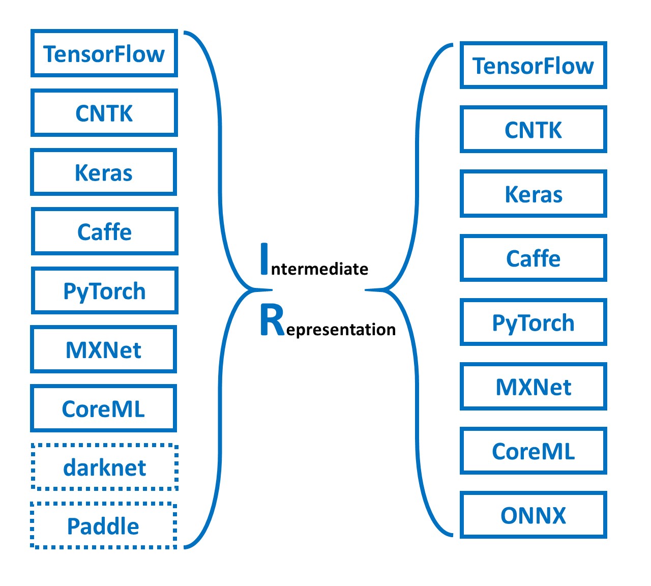
MMdnn主要有以下特征:
- 模型文件转换器,不同的框架间转换DNN模型
- 模型代码片段生成器,生成适合不同框架的代码
- 模型可视化,DNN网络结构和框架参数可视化
- 模型兼容性测试(正在进行中)
【04/06/2018】
Dataset:
Introduce:
Visual Object Classes Challenge 2012 (VOC2012)
PASCAL‘s full name is Pattern Analysis, Statistical Modelling and Computational Learning.
VOC’s full name is Visual OBject Classes.
The first competition was held in 2005 and terminated in 2012. I will use the last updated dataset which is VOC2012 dataset.
The main aim of this competition is object detection, there are 20 classes objects in the dataset:
- person
- bird, cat, cow, dog, horse, sheep
- aeroplane, bicycle, boat, bus, car, motorbike, train
- bottle, chair, dining table, potted plant, sofa, tv/monitor
Detection Task
Referenced:
The PASCAL Visual Object Classes Challenge 2012 (VOC2012) Development Kit
Mark Everingham - John Winn
http://host.robots.ox.ac.uk/pascal/VOC/voc2012/htmldoc/index.html
Task:
For each of the twenty classes predict the bounding boxes of each object of that class in a test image (if any). Each bounding box should be output with an associated real-valued confidence of the detection so that a precision/recall curve can be drawn. Participants may choose to tackle all, or any subset of object classes, for example ‘cars only’ or ‘motorbikes and cars’.
Competitions:
Two competitions are defined according to the choice of training data:
- taken from the $VOC_{trainval}$ data provided.
- from any source excluding the $VOC_{test}$ data provided.
Submission of Results:
A separate text file of results should be generated for each competition and each class e.g. `car’. Each line should be a detection output by the detector in the following format:
1
<image identifier> <confidence> <left> <top> <right> <bottom>
where (left,top)-(right,bottom) defines the bounding box of the detected object. The top-left pixel in the image has coordinates $(1,1)$. Greater confidence values signify greater confidence that the detection is correct. An example file excerpt is shown below. Note that for the image 2009_000032, multiple objects are detected:1
2
3
4
5
6
7comp3_det_test_car.txt:
...
2009_000026 0.949297 172.000000 233.000000 191.000000 248.000000
2009_000032 0.013737 1.000000 147.000000 114.000000 242.000000
2009_000032 0.013737 1.000000 134.000000 94.000000 168.000000
2009_000035 0.063948 455.000000 229.000000 491.000000 243.000000
...
Evaluation:
The detection task will be judged by the precision/recall curve. The principal quantitative measure used will be the average precision (AP). Detections are considered true or false positives based on the area of overlap with ground truth bounding boxes. To be considered a correct detection, the area of overlap $a_o$ between the predicted bounding box $B_p$ and ground truth bounding box $B_{gt}$ must exceed $50\%$ by the formula:
XML标注格式
对于目标检测来说,每一张图片对应一个xml格式的标注文件。所以你会猜到,就像gemfield准备的训练集有8万张照片一样,在存放xml文件的目录里,这里也将会有8万个xml文件。下面是其中一个xml文件的示例:
1
2
3
4
5
6
7
8
9
10
11
12
13
14
15
16
17
18
19
20
21
22
23
24
25
26
27
28
29
30
31
32
33 <?xml version="1.0" encoding="utf-8"?>
<annotation>
<folder>VOC2007</folder>
<filename>test100.mp4_3380.jpeg</filename>
<size>
<width>1280</width>
<height>720</height>
<depth>3</depth>
</size>
<object>
<name>gemfield</name>
<bndbox>
<xmin>549</xmin>
<xmax>715</xmax>
<ymin>257</ymin>
<ymax>289</ymax>
</bndbox>
<truncated>0</truncated>
<difficult>0</difficult>
</object>
<object>
<name>civilnet</name>
<bndbox>
<xmin>842</xmin>
<xmax>1009</xmax>
<ymin>138</ymin>
<ymax>171</ymax>
</bndbox>
<truncated>0</truncated>
<difficult>0</difficult>
</object>
<segmented>0</segmented>
</annotation>
在这个测试图片上,我们标注了2个object,一个是gemfield,另一个是civilnet。
在这个xml例子中:
- bndbox是一个轴对齐的矩形,它框住的是目标在照片中的可见部分;
- truncated表明这个目标因为各种原因没有被框完整(被截断了),比如说一辆车有一部分在画面外;
- occluded是说一个目标的重要部分被遮挡了(不管是被背景的什么东西,还是被另一个待检测目标遮挡);
- difficult表明这个待检测目标很难识别,有可能是虽然视觉上很清楚,但是没有上下文的话还是很难确认它属于哪个分类;标为difficult的目标在测试成绩的评估中一般会被忽略。
注意:在一个object中,name 标签要放在前面,否则的话,目标检测的一个重要工程实现SSD会出现解析数据集错误(另一个重要工程实现py-faster-rcnn则不会)。
【07/06/2018】
Poster conference

5 People in one group to present their object.
I present this object to my supervisor in this conference.
【11/06/2018】
R-CNN
Paper: Rich feature hierarchies for accurate object detection and semantic segmentation
【论文主要特点】(相对传统方法的改进)
- 速度: 经典的目标检测算法使用滑动窗法依次判断所有可能的区域。本文则(采用Selective Search方法)预先提取一系列较可能是物体的候选区域,之后仅在这些候选区域上(采用CNN)提取特征,进行判断。
- 训练集: 经典的目标检测算法在区域中提取人工设定的特征。本文则采用深度网络进行特征提取。使用两个数据库: 一个较大的识别库 (ImageNet ILSVC 2012):标定每张图片中物体的类别。一千万图像,1000类。 一个较小的检测库(PASCAL VOC 2007):标定每张 图片中,物体的类别和位置,一万图像,20类。 本文使用识别库进行预训练得到CNN(有监督预训练),而后用检测库调优参数,最后在 检测库上评测。
【流程】
- 候选区域生成: 一张图像生成1K~2K个候选区域 (采用Selective Search 方法)
- 特征提取: 对每个候选区域,使用深度卷积网络提取特征 (CNN)
- 类别判断: 特征送入每一类的SVM 分类器,判别是否属于该类
- 位置精修: 使用回归器精细修正候选框位置

- 使用一种过分割手段,将图像分割成小区域 (1k~2k 个)
- 查看现有小区域,按照合并规则合并可能性最高的相邻两个区域。重复直到整张图像合并成一个区域位置
- 输出所有曾经存在过的区域,所谓候选区域
其中合并规则如下: 优先合并以下四种区域:- 颜色(颜色直方图)相近的
- 纹理(梯度直方图)相近的
- 合并后总面积小的: 保证合并操作的尺度较为均匀,避免一个大区域陆续“吃掉”其他小区域 (例:设有区域a-b-c-d-e-f-g-h。较好的合并方式是:ab-cd-ef-gh -> abcd-efgh -> abcdefgh。 不好的合并方法是:ab-c-d-e-f-g-h ->abcd-e-f-g-h ->abcdef-gh -> abcdefgh)
- 合并后,总面积在其BBOX中所占比例大的: 保证合并后形状规则。
【12/06/2018】
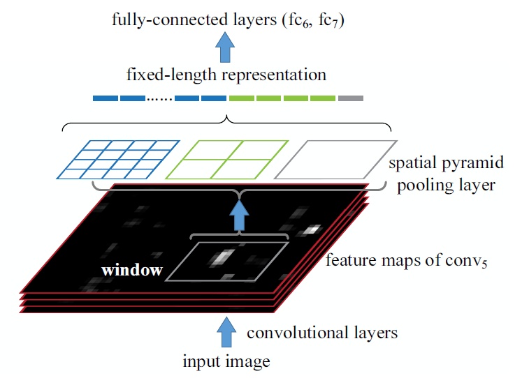
SPP-CNN
Paper: Spatial Pyramid Pooling in Deep Convolutional Networks for Visual Recognition
【论文主要特点】(相对传统方法的改进)
RCNN使用CNN作为特征提取器,首次使得目标检测跨入深度学习的阶段。但是RCNN对于每一个区域候选都需要首先将图片放缩到固定的尺寸(224*224),然后为每个区域候选提取CNN特征。容易看出这里面存在的一些性能瓶颈:
- 速度瓶颈:重复为每个region proposal提取特征是极其费时的,Selective Search对于每幅图片产生2K左右个region proposal,也就是意味着一幅图片需要经过2K次的完整的CNN计算得到最终的结果。
- 性能瓶颈:对于所有的region proposal防缩到固定的尺寸会导致我们不期望看到的几何形变,而且由于速度瓶颈的存在,不可能采用多尺度或者是大量的数据增强去训练模型。
【流程】
- 首先通过selective search产生一系列的region proposal
- 然后训练多尺寸识别网络用以提取区域特征,其中处理方法是每个尺寸的最短边大小在尺寸集合中:
$s \in S = {480,576,688,864,1200}$
训练的时候通过上面提到的多尺寸训练方法,也就是在每个epoch中首先训练一个尺寸产生一个model,然后加载这个model并训练第二个尺寸,直到训练完所有的尺寸。空间金字塔池化使用的尺度为:1*1,2*2,3*3,6*6,一共是50个bins。 - 在测试时,每个region proposal选择能使其包含的像素个数最接近224*224的尺寸,提取相 应特征。
- 训练SVM,BoundingBox回归.
【13/06/2018】
FAST R-CNN
Paper: Fast R-CNN
【论文主要特点】(相对传统方法的改进)
- 测试时速度慢:RCNN一张图像内候选框之间大量重叠,提取特征操作冗余。本文将整张图像归一化后直接送入深度网络。在邻接时,才加入候选框信息,在末尾的少数几层处理每个候选框。
- 训练时速度慢 :原因同上。在训练时,本文先一张图像送入网络,紧接着送入从这幅图像上提取出的候选区域。这些候选区域的前几层特征不需要再重复计算。
- 训练所需空间大: RCNN中独立的分类器和回归器需要大量特征作为训练样本。本文把类别判断和位置精调统一用深度网络实现,不再需要额外存储。
【流程】
- 网络首先用几个卷积层(conv)和最大池化层处理整个图像以产生conv特征图。
- 然后,对于每个对象建议框(object proposals ),感兴趣区域(region of interest——RoI)池层从特征图提取固定长度的特征向量。
- 每个特征向量被输送到分支成两个同级输出层的全连接(fc)层序列中:
其中一层进行分类,对 目标关于K个对象类(包括全部“背景background”类)产生softmax概率估计,即输出每一个RoI的概率分布;
另一层进行bbox regression,输出K个对象类中每一个类的四个实数值。每4个值编码K个类中的每个类的精确边界盒(bounding-box)位置,即输出每一个种类的的边界盒回归偏差。整个结构是使用多任务损失的端到端训练(trained end-to-end with a multi-task loss)。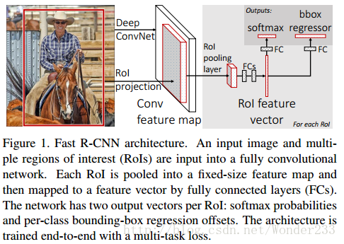
【14~18/06/2018】
FASTER R-CNN
I want to use Faster R-cnn as the first method to implement object detection system.
Paper: Faster R-CNN: Towards Real-Time Object Detection with Region Proposal Networks
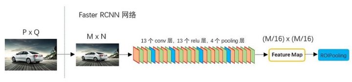
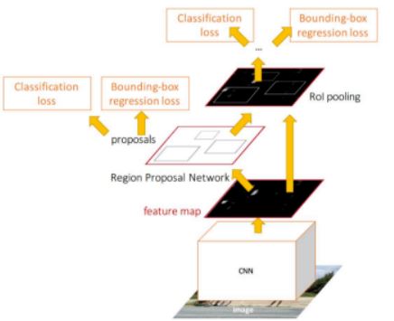
在结构上,Faster RCNN已经将特征抽取(feature extraction),proposal提取,bounding box regression(rect refine),classification都整合在了一个网络中,使得综合性能有较大提高,在检测速度方面尤为明显。
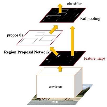
流程
- Conv layers:作为一种CNN网络目标检测方法,Faster R-CNN首先使用一组基础的conv+relu+pooling层提取image的feature maps。该feature maps被共享用于后续RPN层和全连接层。
- Region Proposal Networks:RPN网络用于生成region proposals。该层通过softmax判断anchors属于foreground或者background,再利用bounding box regression修正anchors获得精确的proposals。
- Roi Pooling:该层收集输入的feature maps和proposals,综合这些信息后提取proposal feature maps,送入后续全连接层判定目标类别。
- Classification:利用proposal feature maps计算proposal的类别,同时再次bounding box regression获得检测框最终的精确位置。
解释
[1. Conv layers]
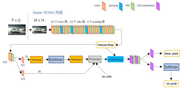
Conv layers包含了conv,pooling,relu三种层。以python版本中的VGG16模型中的faster_rcnn_test.pt的网络结构为例,如图, Conv layers部分共有13个conv层,13个relu层,4个pooling层。这里有一个非常容易被忽略但是又无比重要的信息,在Conv layers中:
- 所有的conv层都是: $kernel_size=3$ , $pad=1$ , $stride=1$
所有的pooling层都是: $kernel_size=2$ , $pad=0$ , $stride=2$
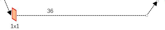
为何重要?在Faster RCNN Conv layers中对所有的卷积都做了扩边处理( $pad=1$ ,即填充一圈0),导致原图变为 $(M+2)\times (N+2)$ 大小,再做3x3卷积后输出 $M\times N$ 。正是这种设置,导致Conv layers中的conv层不改变输入和输出 矩阵大小。如下图:
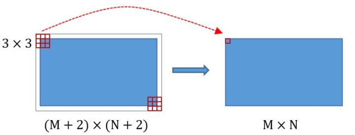
类似的是,Conv layers中的pooling层 $kernel_size=2$ , $stride=2$ 。这样每个经过pooling层的 $M\times N$ 矩阵,都会变为 $(M/2) \times(N/2)$ 大小。综上所述,在整个Conv layers中,conv和relu层不改变输入输出大小,只有pooling层使输出长宽都变为输入的1/2。
那么,一个 $M\times N$ 大小的矩阵经过Conv layers固定变为 $(M/16)\times (N/16)$ !这样Conv layers生成的featuure map中都可以和原图对应起来。
[2. Region Proposal Networks(RPN)]
经典的检测方法生成检测框都非常耗时,如OpenCV adaboost使用滑动窗口+图像金字塔生成检测框;或如R-CNN使用SS(Selective Search)方法生成检测框。而Faster RCNN则抛弃了传统的滑动窗口和SS方法,直接使用RPN生成检测框,这也是Faster R-CNN的巨大 优势,能极大提升检测框的生成速度。
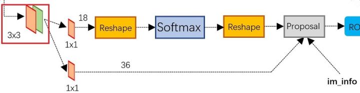
上图展示了RPN网络的具体结构。可以看到RPN网络实际分为2条线,上面一条通过softmax分类anchors获得foreground和 background(检测目标是foreground),下面一条用于计算对于anchors的bounding box regression偏移量,以获得精确的 proposal。而最后的Proposal层则负责综合foreground anchors和bounding box regression偏移量获取proposals,同时剔除太 小和超出边界的proposals。其实整个网络到了Proposal Layer这里,就完成了相当于目标定位的功能。
2.1 多通道图像卷积基础知识介绍
- 对于单通道图像+单卷积核做卷积,之前展示了;
对于多通道图像+多卷积核做卷积,计算方式如下:
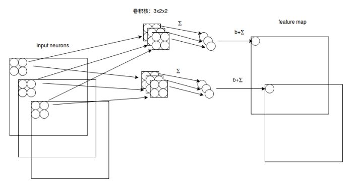
输入有3个通道,同时有2个卷积核。对于每个卷积核,先在输入3个通道分别作卷积,再将3个通道结果加起来得到卷积输出。所以对 于某个卷积层,无论输入图像有多少个通道,输出图像通道数总是等于卷积核数量!
对多通道图像做 $1\times1$ 卷积,其实就是将输入图像于每个通道乘以卷积系数后加在一起,即相当于把原图像中本来各个独立的 通道“联通”在了一起。
2.2 Anchors
提到RPN网络,就不能不说anchors。所谓anchors,实际上就是一组由rpn/generate_anchors.py生成的矩形。直接运行作者demo中 的generate_anchors.py可以得到以下输出:
[[ -84. -40. 99. 55.]
[-176. -88. 191. 103.]
[-360. -184. 375. 199.]
[ -56. -56. 71. 71.]
[-120. -120. 135. 135.]
[-248. -248. 263. 263.]
[ -36. -80. 51. 95.]
[ -80. -168. 95. 183.]
[-168. -344. 183. 359.]]
其中每行的4个值 $(x1,y1,x2,y2)$ 代表矩形左上和右下角点坐标。9个矩形共有3种形状,长宽比为大约为 $width:height = [1:1, 1:2, 2:1]$ 三种,如下图。实际上通过anchors就引入了检测中常用到的多尺度方法。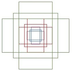
注:关于上面的anchors size,其实是根据检测图像设置的。在python demo中,会把任意大小的输入图像reshape成 $800\times600$。再回头来看anchors的大小,anchors中长宽 1:2 中最大为 $352\times704$ ,长宽 2:1 中最大 $736\times384$ ,基本是cover了 $800\times600$ 的各个尺度和形状。
那么这9个anchors是做什么的呢?借用Faster RCNN论文中的原图,如下图,遍历Conv layers计算获得的feature maps,为每一个点都配备这9种anchors作为初始的检测框。这样做获得检测框很不准确,不用担心,后面还有2次bounding box regression可以修正检测框位置。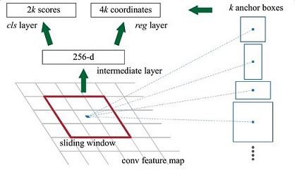
解释一下上面这张图的数字。
- 在原文中使用的是ZF model中,其Conv Layers中最后的conv5层num_output=256,对应生成256张特征图,所以相当于feature map每个点都是256-dimensions
- 在conv5之后,做了rpn_conv/3x3卷积且num_output=256,相当于每个点又融合了周围3x3的空间信息(猜测这样做也许更鲁棒?反正我没测试),同时256-d不变(如图4和图7中的红框)
- 假设在conv5 feature map中每个点上有k个anchor(默认k=9),而每个anhcor要分foreground和background,所以每个点由256d feature转化为cls=2k scores;而每个anchor都有[x, y, w, h]对应4个偏移量,所以reg=4k coordinates
补充一点,全部anchors拿去训练太多了,训练程序会在合适的anchors中随机选取128个postive anchors+128个negative anchors进行训练(什么是合适的anchors下文5.1有解释)
2.3 softmax判定foreground与background
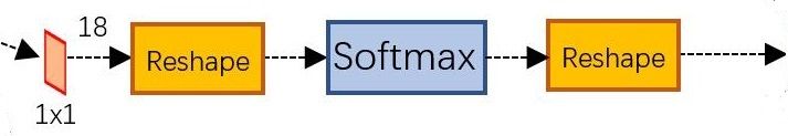
一副MxN大小的矩阵送入Faster RCNN网络后,到RPN网络变为(M/16)x(N/16),不妨设 W=M/16 , H=N/16 。在进入reshape与softmax之前,先做了1x1卷积,如下图:
该1x1卷积的caffe prototxt定义如下:
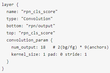
可以看到其num_output=18,也就是经过该卷积的输出图像为 $W\times H \times 18$ 大小(注意第二章开头提到的卷积计算方式)。这也就刚好对应了feature maps每一个点都有9个anchors,同时每个anchors又有可能是foreground和background,所有这些信息都保存 $W\times H\times (9\cdot2)$ 大小的矩阵。为何这样做?后面接softmax分类获得foreground anchors,也就相当于初步提取了检测目标候选区域box(一般认为目标在foreground anchors中)。
综上所述,RPN网络中利用anchors和softmax初步提取出foreground anchors作为候选区域。2.4 bounding box regression原理
如图所示绿色框为飞机的Ground Truth(GT),红色为提取的foreground anchors,即便红色的框被分类器识别为飞机,但是由于红色的框定位不准,这张图相当于没有正确的检测出飞机。所以我们希望采用一种方法对红色的框进行微调,使得foreground anchors和GT更加接近。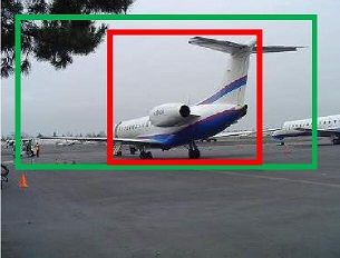
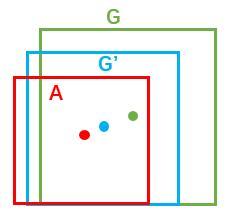
对于窗口一般使用四维向量 (x, y, w, h) 表示,分别表示窗口的中心点坐标和宽高。对于下图,红色的框A代表原始的Foreground Anchors,绿色的框G代表目标的GT,我们的目标是寻找一种关系,使得输入原始的anchor A经过映射得到一个跟真实窗口G更接近的回归窗口G’,即:- 给定:$anchor A=(A_{x}, A_{y}, A_{w}, A_{h})$ 和 $GT=[G_{x}, G_{y}, G_{w}, G_{h}]$
寻找一种变换F,使得:$F(A_{x}, A_{y}, A_{w}, A_{h})=(G_{x}^{‘}, G_{y}^{‘}, G_{w}^{‘}, G_{h}^{‘})$,其中 $(G_{x}^{‘}, G_{y}^{‘}, G_{w}^{‘}, G_{h}^{‘}) \approx (G_{x}, G_{y}, G_{w}, G_{h})$
那么经过何种变换F才能从图10中的anchor A变为G’呢? 比较简单的思路就是:先做平移
$G^{‘}{x} = A{w} \cdot d_{x}(A) + A_{x} $
$G^{‘}{y} = A{y} \cdot d_{y}(A) + A_{y} $- 再做缩放
$G^{‘}{w} = A{w} \cdot exp(d_{w}(A)) $
$G^{‘}{h} = A{h} \cdot exp(d_{h}(A)) $
观察上面4个公式发现,需要学习的是 $d_{x}(A),d_{y}(A),d_{w}(A),d_{h}(A)$ 这四个变换。当输入的anchor A与GT相差较小时,可以认为这种变换是一种线性变换, 那么就可以用线性回归来建模对窗口进行微调(注意,只有当anchors A和GT比较接近时,才能使用线性回归模型,否则就是复杂的非线性问题了)。
接下来的问题就是如何通过线性回归获得 $d_{x}(A),d_{y}(A),d_{w}(A),d_{h}(A)$ 了。线性回归就是给定输入的特征向量X, 学习一组参数W, 使得经过线性回归后的值跟真实值Y非常接近,即$Y=WX$。对于该问题,输入X是cnn feature map,定义为Φ;同时还有训练传入A与GT之间的变换量,即$(t_{x}, t_{y}, t_{w}, t_{h})$。输出是$d_{x}(A),d_{y}(A),d_{w}(A),d_{h}(A)$四个变换。那么目标函数可以表示为:
$d_{}(A) = w^{T}_{} \cdot \phi(A)$
其中Φ(A)是对应anchor的feature map组成的特征向量,w是需要学习的参数,d(A)是得到的预测值(*表示 x,y,w,h,也就是每一个变换对应一个上述目标函数)。为了让预测值$(t_{x}, t_{y}, t_{w}, t_{h})$与真实值差距最小,设计损失函数:
$Loss = \sum^{N}{i}(t^{i}{} - \hat{w}^{T}_{} \cdot \phi(A^{i}))^{2}$
函数优化目标为:
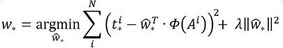
需要说明,只有在GT与需要回归框位置比较接近时,才可近似认为上述线性变换成立。
说完原理,对应于Faster RCNN原文,foreground anchor与ground truth之间的平移量 $(t_x, t_y)$ 与尺度因子 $(t_w, t_h)$ 如下:
对于训练bouding box regression网络回归分支,输入是cnn feature Φ,监督信号是Anchor与GT的差距 $(t_x, t_y, t_w, t_h)$,即训练目标是:输入Φ的情况下使网络输出与监督信号尽可能接近。
那么当bouding box regression工作时,再输入Φ时,回归网络分支的输出就是每个Anchor的平移量和变换尺度 $(t_x, t_y, t_w, t_h)$,显然即可用来修正Anchor位置了。
2.5 对proposals进行bounding box regression
在了解bounding box regression后,再回头来看RPN网络第二条线路,如下图。
其 $num_output=36$ ,即经过该卷积输出图像为 $W\times H\times 36$ ,在caffe blob存储为 [1, 36, H, W] ,这里相当于feature maps每个点都有9个anchors,每个anchors又都有4个用于回归的$d_{x}(A),d_{y}(A),d_{w}(A),d_{h}(A)$变换量。
2.6 Proposal Layer
Proposal Layer负责综合所有 $d_{x}(A),d_{y}(A),d_{w}(A),d_{h}(A)$ 变换量和foreground anchors,计算出精准的proposal,送入后续RoI Pooling Layer。
首先解释im_info。对于一副任意大小PxQ图像,传入Faster RCNN前首先reshape到固定 $M\times N$ ,im_info=[M, N, scale_factor]则保存了此次缩放的所有信息。然后经过Conv Layers,经过4次pooling变为 $W\times H=(M/16)\times(N/16)$ 大小,其中feature_stride=16则保存了该信息,用于计算anchor偏移量。
Proposal Layer forward(caffe layer的前传函数)按照以下顺序依次处理:
- 生成anchors,利用$[d_{x}(A),d_{y}(A),d_{w}(A),d_{h}(A)]$对所有的anchors做bbox regression回归(这里的anchors生成和训练时完全一致)
- 按照输入的foreground softmax scores由大到小排序anchors,提取前pre_nms_topN(e.g. 6000)个anchors,即提取修正位置后的foreground anchors。
- 限定超出图像边界的foreground anchors为图像边界(防止后续roi pooling时proposal超出图像边界)
- 剔除非常小(width<threshold or height<threshold)的foreground anchors
- 进行nonmaximum suppression
- 再次按照nms后的foreground softmax scores由大到小排序fg anchors,提取前post_nms_topN(e.g. 300)结果作为proposal输出。
之后输出 proposal=[x1, y1, x2, y2] ,注意,由于在第三步中将anchors映射回原图判断是否超出边界,所以这里输出的proposal是对应 $M\times N$ 输入图像尺度的,这点在后续网络中有用。另外我认为,严格意义上的检测应该到此就结束了,后续部分应该属于识别了~
RPN网络结构就介绍到这里,总结起来就是:
生成anchors -> softmax分类器提取fg anchors -> bbox reg回归fg anchors -> Proposal Layer生成proposals
【19/06/2018】
处理 XML 文档
使用 xml.etree.ElementTree 这个包去解析XML文件, 并且整理成为list形式
【流程】
- 读取XML文件
- 区分训练集测试集根据竞赛要求
- 解析XML文档收录到PYTHON词典中
Github 的 jupyter notebook 地址
训练集根据竞赛的 trainval.txt 文件给的图片作为训练集
其余的作为训练集
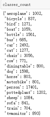
解析后, 总共有 17125 张图片,
其中 11540 张作为训练集
图片中的20个类的统计情况:
【20/06/2018】
根据信息画出BBOXES
安装 cv2 这个包
1
pip install opencv-python
注意: OpenCV-python 中颜色格式 是BGR 而不是 RGB
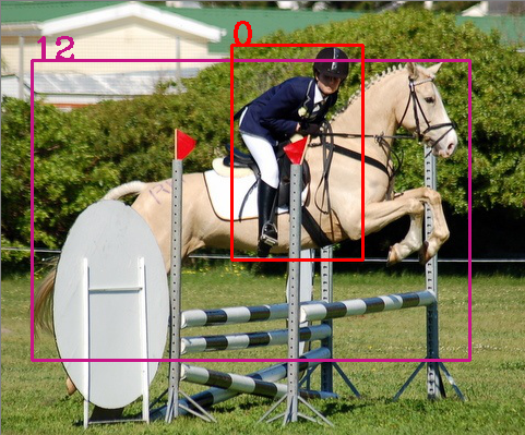
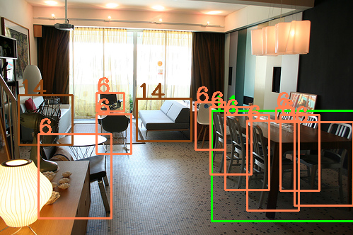
在VOC2012数据集里面,总共有20类, 根据不同的种类用不同的颜色和唯一的编码画BBOXES。
| class | class_mapping | BGR of bbox |
|---|---|---|
| Person | 0 | (0, 0, 255) |
| Aeroplane | 1 | (0, 0, 255) |
| Tvmonitor | 2 | (0, 128, 0) |
| Train | 3 | (128, 128, 128) |
| Boat | 4 | (0, 165, 255) |
| Dog | 5 | (0, 255, 255) |
| Chair | 6 | (80, 127, 255) |
| Bird | 7 | (208, 224, 64) |
| Bicycle | 8 | (235, 206, 135) |
| Bottle | 9 | (128, 0, 0) |
| Sheep | 10 | (140, 180, 210) |
| Diningtable | 11 | (0, 255, 0) |
| Horse | 12 | (133, 21, 199) |
| Motorbike | 13 | (47, 107, 85) |
| Sofa | 14 | (19, 69, 139) |
| Cow | 15 | (222, 196, 176) |
| Car | 16 | (0, 0, 0) |
| Cat | 17 | (225, 105, 65) |
| Bus | 18 | (255, 255, 255) |
| Pottedplant | 19 | (205, 250, 255) |
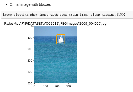
我写了一个show_image_with_bbox函数去画出带BBOXES的图根据处理XML文件得到的list:
Github 的 jupyter notebook 地址
EXAMPLE:
【21/06/2018】
config setting
set config class:
for image enhancement:
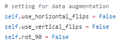
image enhancement
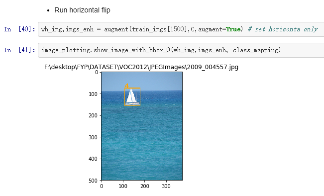
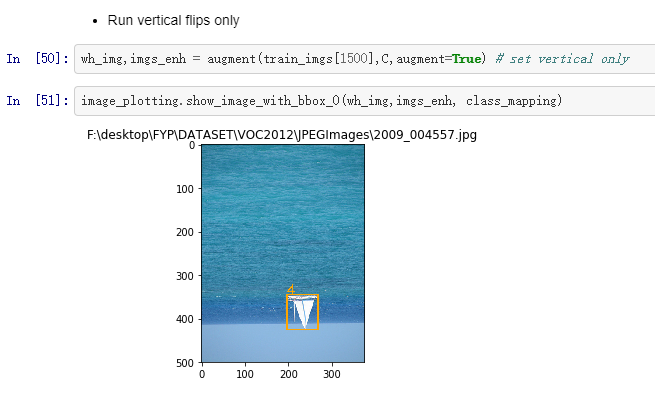
According to the config of three peremeters, users could augment image with 3 different ways or using them all.
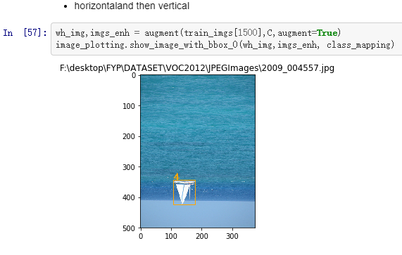
For horizontal and vertical flips, 1/3 probability to triggle
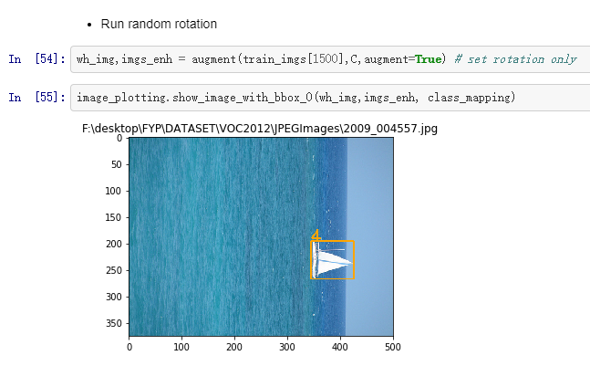
With 0,90,180,270 rotation,
This function could increase the number of datasets.
image flips and rotation are realized by opencv and replace of height and width
New cordinates of bboxes are calculated acccording to different change of image
detailed in Github, jupyter notebook: address
Orignal image:
horizontal flip:
Vertical filp:
Random rotation:
Horizontal and then vertical flips:
【22/06/2018】
Image rezise
This function is to rezise input image to a uniform size with same shortest side
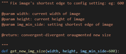
According to set the value of shortest side, convergent-divergent or augmented another side proportion
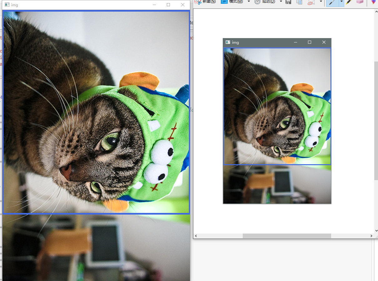
Test:
Left image is resized image, in this case, the orignal image amplified.
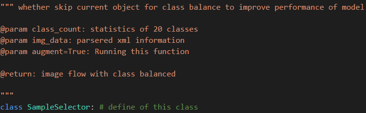
Class Balance
When training the model, if we sent image with no repeating classes, it may help to improve the performance of model. Therefore, this function is to make sure no repeating classes in two closed input image.
Test:
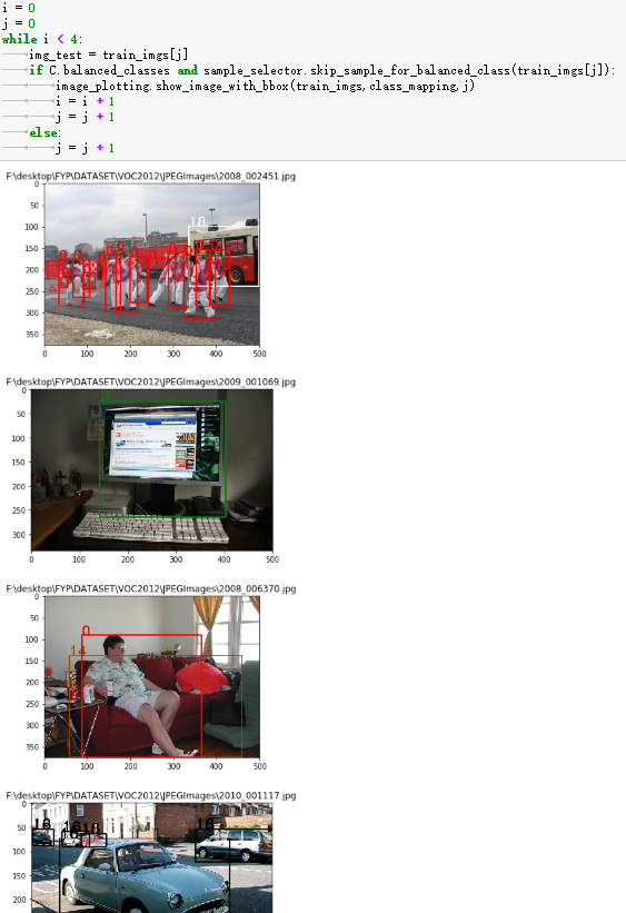
Random output 4 iamge with is function, it could find no repeating classes in two closed image. However, it may reduce the number of trainning image because skip some images.
【25~26/06/2018】
Region Proposal Networks(RPN)
可以看到RPN网络实际分为2条线,上面一条通过softmax分类anchors获得foreground和background(检测目标是foreground),下面一条用于计算对于anchors的bounding box regression偏移量,以获得精确的proposal。而最后的Proposal层则负责综合foreground anchors和bounding box regression偏移量获取proposals,同时剔除太小和超出边界的proposals。其实整个网络到了Proposal Layer这里,就完成了相当于目标定位的功能。
Anchors
对每一个点生成的矩形
其中每行的4个值 (x1,y1,x2,y2) 代表矩形左上和右下角点坐标。9个矩形共有3种形状,长宽比为大约为 width:height = [1:1, 1:2, 2:1]
通过遍历Conv layers计算获得的feature maps,为每一个点都配备这9种anchors作为初始的检测框。这样做获得检测框很不准确,不用担心,后面还有2次bounding box regression可以修正检测框位置.
Code
1 | """ intersection of two bboxes |
1 | """ union of two bboxes |
1 | """ calculate ratio of intersection and union |
IOU is used to bounding box regression
rpn calculation
- Traversal all pre-anchors to calculate IOU with GT bboxes
- Set number and proprty of pre-anchors
- return specity number of result(Anchors)
1 | """ |
【注:其只会返回num_regions(这里设置为256)个有效的正负样本 】
【流程】
Initialise paramters: see jupyter notebook
Calculate the size of map feature:1
(output_width, output_height) = img_length_calc_function(resized_width, resized_height)
Get the GT box coordinates, and resize to account for image resizing
after rezised functon, the coordinates of bboxes need to re-calculation:1
2
3
4
5for bbox_num, bbox in enumerate(img_data['bboxes']):
gta[bbox_num, 0] = bbox['x1'] * (resized_width / float(width))
gta[bbox_num, 1] = bbox['x2'] * (resized_width / float(width))
gta[bbox_num, 2] = bbox['y1'] * (resized_height / float(height))
gta[bbox_num, 3] = bbox['y2'] * (resized_height / float(height))
【注意gta的存储形式是(x1,x2,y1,y2)而不是(x1,y1,x2,y2)】
Traverse all possible group of sizes
anchor box scales [128, 256, 512]
anchor box ratios [1:1,1:2,2:1]1
2
3
4for anchor_size_idx in range(len(anchor_sizes)):
for anchor_ratio_idx in range(len(anchor_ratios)):
anchor_x = anchor_sizes[anchor_size_idx] * anchor_ratios[anchor_ratio_idx][0]
anchor_y = anchor_sizes[anchor_size_idx] * anchor_ratios[anchor_ratio_idx][1]
Traver one bbox group, all pre boxes generated by anchors
output_width,output_height:width and height of map feature
downscale:mapping ration, defualt 16
if to delete box out of iamge
1 | for ix in range(output_width): |
【注:现在我们确定了一个预选框组合有确定了中心点那就是唯一确定一个框了,接下来就是来确定这个宽的性质了:是否包含物体、如包含物体其回归梯度是多少】
要确定以上两个性质,每一个框都需要遍历图中的所有bboxes 然后计算该预选框与bbox的交并比(IOU)
如果现在的交并比curr_iou大于该bbox最好的交并比或者大于给定的阈值则求下列参数,这些参数是后来要用的即回归梯度
tx:两个框中心的宽的距离与预选框宽的比
ty:同tx
tw:bbox的宽与预选框宽的比
th:同理
1 | if curr_iou > best_iou_for_bbox[bbox_num] or curr_iou > C.rpn_max_overlap: |
对应于Faster RCNN原文,foreground anchor与ground truth之间的平移量 $(t_x, t_y)$ 如下:

对于训练bouding box regression网络回归分支,输入是cnn feature Φ,监督信号是Anchor与GT的差距 $(t_x, t_y, t_w, t_h)$,即训练目标是:输入 Φ的情况下使网络输出与监督信号尽可能接近。
那么当bouding box regression工作时,再输入Φ时,回归网络分支的输出就是每个Anchor的平移量和变换尺度 $(t_x, t_y, t_w, t_h)$,显然即可用来修正Anchor位置了。
如果相交的不是背景,那么进行一系列更新
关于bbox的相关信息更新
预选框的相关更新:如果交并比大于阈值这是pos
best_iou_for_loc:其记录的是有最大交并比为多少和其对应的回归梯度
num_anchors_for_bbox[bbox_num]:记录的是bbox拥有的pos预选框的个数
如果小于最小阈值是neg,在这两个之间是neutral
需要注意的是:判断一个框为neg需要其与所有的bbox的交并比都小于最小的阈值
1 | if img_data['bboxes'][bbox_num]['class'] != 'bg': |
当结束对所有的bbox的遍历时,来确定该预选宽的性质。
y_is_box_valid:该预选框是否可用(nertual就是不可用的)
y_rpn_overlap:该预选框是否包含物体
y_rpn_regr:回归梯度1
2
3
4
5
6
7
8
9
10
11if bbox_type == 'neg':
y_is_box_valid[jy, ix, anchor_ratio_idx + n_anchratios * anchor_size_idx] = 1
y_rpn_overlap[jy, ix, anchor_ratio_idx + n_anchratios * anchor_size_idx] = 0
elif bbox_type == 'neutral':
y_is_box_valid[jy, ix, anchor_ratio_idx + n_anchratios * anchor_size_idx] = 0
y_rpn_overlap[jy, ix, anchor_ratio_idx + n_anchratios * anchor_size_idx] = 0
else:
y_is_box_valid[jy, ix, anchor_ratio_idx + n_anchratios * anchor_size_idx] = 1
y_rpn_overlap[jy, ix, anchor_ratio_idx + n_anchratios * anchor_size_idx] = 1
start = 4 * (anchor_ratio_idx + n_anchratios * anchor_size_idx)
y_rpn_regr[jy, ix, start:start+4] = best_regr
如果有一个bbox没有pos的预选宽和其对应,这找一个与它交并比最高的anchor的设置为pos1
2
3
4
5
6
7
8
9for idx in range(num_anchors_for_bbox.shape[0]):
if num_anchors_for_bbox[idx] == 0:
# no box with an IOU greater than zero ...
if best_anchor_for_bbox[idx, 0] == -1:
continue
y_is_box_valid[best_anchor_for_bbox[idx,0], best_anchor_for_bbox[idx,1], best_anchor_for_bbox[idx,2] + n_anchratios *best_anchor_for_bbox[idx,3]] = 1
y_rpn_overlap[best_anchor_for_bbox[idx,0], best_anchor_for_bbox[idx,1], best_anchor_for_bbox[idx,2] + n_anchratios *best_anchor_for_bbox[idx,3]] = 1
start = 4 * (best_anchor_for_bbox[idx,2] + n_anchratios * best_anchor_for_bbox[idx,3])
y_rpn_regr[best_anchor_for_bbox[idx,0], best_anchor_for_bbox[idx,1], start:start+4] = best_dx_for_bbox[idx, :]
将深度变到第一位,给向量增加一个维度, 在Tensorflow中, 第一纬度是batch size, 此外, 变换向量位置匹配要求1
2
3
4
5
6
7
8y_rpn_overlap = np.transpose(y_rpn_overlap, (2, 0, 1))
y_rpn_overlap = np.expand_dims(y_rpn_overlap, axis=0)
y_is_box_valid = np.transpose(y_is_box_valid, (2, 0, 1))
y_is_box_valid = np.expand_dims(y_is_box_valid, axis=0)
y_rpn_regr = np.transpose(y_rpn_regr, (2, 0, 1))
y_rpn_regr = np.expand_dims(y_rpn_regr, axis=0)
从可用的预选框中选择num_regions
如果pos的个数大于num_regions / 2,则将多下来的地方置为不可用。如果小于pos不做处理
接下来将pos与neg总是超过num_regions个的neg预选框置为不可用
最后, 256个预选框,128个positive,128个negative 会生成 在一张图片里面1
2
3
4
5
6
7
8
9
10
11
12pos_locs = np.where(np(y_rpn_overlap[0, :, :, :] =.logical_and= 1, y_is_box_valid[0, :, :, :] == 1))
neg_locs = np.where(np.logical_and(y_rpn_overlap[0, :, :, :] == 0, y_is_box_valid[0, :, :, :] == 1))
num_regions = 256
if len(pos_locs[0]) > num_regions / 2:
val_locs = random.sample(range(len(pos_locs[0])), len(pos_locs[0]) - num_regions / 2)
y_is_box_valid[0, pos_locs[0][val_locs], pos_locs[1][val_locs], pos_locs[2][val_locs]] = 0
num_pos = num_regions / 2
if len(neg_locs[0]) + num_pos > num_regions:
val_locs = random.sample(range(len(neg_locs[0])), len(neg_locs[0]) - num_pos)
y_is_box_valid[0, neg_locs[0][val_locs], neg_locs[1][val_locs], neg_locs[2][val_locs]] = 0
【27/06/2018】
project brief
Re organization of Project plan
Anchors Iterative
Integration of privous work:
In each anchor: config file -> rpn_stride = 16 means generate one anchor in 16 pixels
Jupyter Notebook address
【流程】
Function description1
2
3
4
5
6
7
8
9
10
11
12
13
14
15
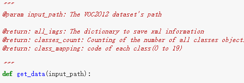
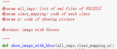
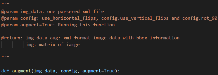
16"""
@param all_img_data: Parsered xml file
@param class_count: Counting of the number of all classes objects
@param C: Configuration class
@param img_length_calc_function: resnet's get_img_output_length() function
@param backend: Tensorflow in this project
#param mode: train or val
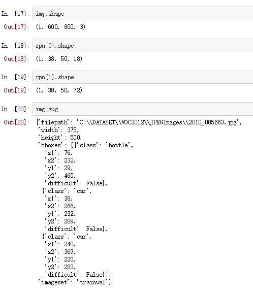
yield np.copy(x_img), [np.copy(y_rpn_cls), np.copy(y_rpn_regr)], img_data_aug
@return: np.copy(x_img): image's matrix data
@return: [np.copy(y_rpn_cls), np.copy(y_rpn_regr)]: calculated rpn class and radient
@return: img_data_aug: correspoding parsed xml information
"""
def get_anchor_gt(all_img_data, class_count, C, img_length_calc_function, backend, mode='train'):
Traverse all input image based on input xml information
- Apply class balance function:
1
2
3
4C.balanced_classes = True
sample_selector = image_processing.SampleSelector(class_count)
if C.balanced_classes and sample_selector.skip_sample_for_balanced_class(img_data):
continue
- Apply image enhance
if input mode is train, apply image enhance to obtain augmented image xml and matrix, if mode is val, obtain image orignal xml and matrix1
2
3
4if mode == 'train':
img_data_aug, x_img = image_enhance.augment(img_data, C, augment=True)
else:
img_data_aug, x_img = image_enhance.augment(img_data, C, augment=False)
verifacation width and hegiht in xml and matrix1
2
3
4(width, height) = (img_data_aug['width'], img_data_aug['height'])
(rows, cols, _) = x_img.shape
assert cols == width
assert rows == height
- Apply rezise function
1
2(resized_width, resized_height) = image_processing.get_new_img_size(width, height, C.im_size)
x_img = cv2.resize(x_img, (resized_width, resized_height), interpolation=cv2.INTER_CUBIC)
- Apply rpn calculation
1
y_rpn_cls, y_rpn_regr = rpn_calculation.calc_rpn(C, img_data_aug, width, height, resized_width, resized_height, img_length_calc_function)
Zero-center by mean pixel, and preprocess image format
BGR -> RGB because when apply resnet, it need RGB but in cv2, it use BGR1
x_img = x_img[:,:, (2, 1, 0)]
For using pre-trainning model, needs to mins mean channel in each dim
1
2
3
4
5x_img = x_img.astype(np.float32)
x_img[:, :, 0] -= C.img_channel_mean[0]
x_img[:, :, 1] -= C.img_channel_mean[1]
x_img[:, :, 2] -= C.img_channel_mean[2]
x_img /= C.img_scaling_factor # default to 1,so no change hereexpand for batch size
1
x_img = np.expand_dims(x_img, axis=0)
for using pre-trainning model, need to sclaling the std to match pre trained model
1
y_rpn_regr[:, y_rpn_regr.shape[1]//2:, :, :] *= C.std_scaling # scaling is 4 here
in tensorflow, sort as batch size, width, height, deep
1
2
3
4if backend == 'tf':
x_img = np.transpose(x_img, (0, 3, 2, 1))
y_rpn_cls = np.transpose(y_rpn_cls, (0, 3, 2, 1))
y_rpn_regr = np.transpose(y_rpn_regr, (0, 3, 2, 1))generator to iteror, using next() to loop
1
yield np.copy(x_img), [np.copy(y_rpn_cls), np.copy(y_rpn_regr)], img_data_aug
【执行】1
2data_gen_train = get_anchor_gt(train_imgs, classes_count, C, nn.get_img_output_length, K.image_dim_ordering(), mode='train')
data_gen_val = get_anchor_gt(val_imgs, classes_count, C, nn.get_img_output_length,K.image_dim_ordering(), mode='val')
Test:1
img,rpn,img_aug = next(data_gen_train)
【28/06/2018】
Resnet50 structure
论文链接: https://arxiv.org/abs/1512.03385
首先,我们要问一个问题:
Is learning better networks as easy as stacking more layers?
很显然不是,原因有二。
一,vanishing/exploding gradients;深度会带来恶名昭著的梯度弥散/爆炸,导致系统不能收敛。然而梯度弥散/爆炸在很大程度上被normalized initialization and intermediate normalization layers处理了。
二、degradation;当深度开始增加的时候,accuracy经常会达到饱和,然后开始下降,但这并不是由于过拟合引起的。可见figure1,56-layer的error大于20-layer的error。
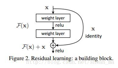
He kaiMing大神认为靠堆layers竟然会导致degradation,那肯定是我们堆的方式不对。因此他提出了一种基于残差块的identity mapping,通过学习残差的方式,而非直接去学习直接的映射关系。
事实证明,靠堆积残差块能够带来很好效果提升。而不断堆积plain layer却会带来很高的训练误差
残差块的两个优点:
1) Our extremely deep residual nets are easy to optimize, but the counterpart “plain” nets (that simply stack layers) exhibit higher training error when the depth increases;
2) Our deep residual nets can easily enjoy accuracy gains from greatly increased depth, producing results substantially better than previous networks.
【29/06/2018】
Resnet50 image structure
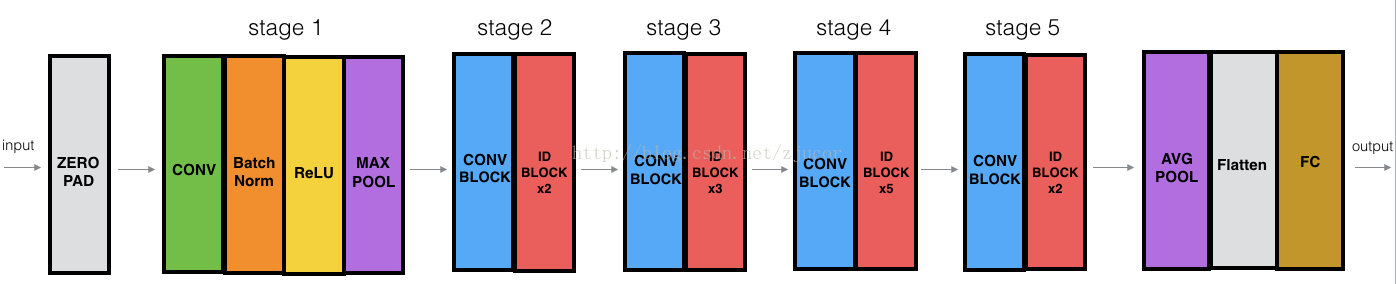
ResNet有2个基本的block,一个是Identity Block,输入和输出的dimension是一样的,所以可以串联多个;另外一个基本block是Conv Block,输入和输出的dimension是不一样的,所以不能连续串联,它的作用本来就是为了改变feature vector的dimension
因为CNN最后都是要把image一点点的convert成很小但是depth很深的feature map,一般的套路是用统一的比较小的kernel(比如VGG都是用3x3),但是随着网络深度的增加,output的channel也增大(学到的东西越来越复杂),所以有必要在进入Identity Block之前,用Conv Block转换一下维度,这样后面就可以连续接Identity Block.
可以看下Conv Block是怎么改变输出维度的: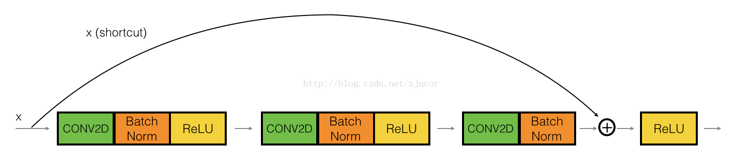
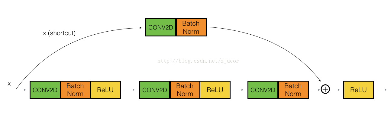
其实就是在shortcut path的地方加上一个conv2D layer(1x1 filter size),然后在main path改变dimension,并与shortcut path对应起来.
July
【02/07/2018】
Construct resnet by keras
残差网络的关键步骤,跨层的合并需要保证x和F(x)的shape是完全一样的,否则它们加不起来。
理解了这一点,我们开始用keras做实现,我们把输入输出大小相同的模块称为identity_block,而把输出比输入小的模块称为conv_block,首先,导入所需的模块:
1 | from keras.models import Model |
我们先来编写identity_block,这是一个函数,接受一个张量为输入,并返回一个张量, 然后是conv层,是有shortcut的:1
2
3
4
5
6
7
8
9
10
11
12
13
14
15
16
17
18
19
20
21
22
23def Conv2d_BN(x, nb_filter,kernel_size, strides=(1,1), padding='same',name=None):
if name is not None:
bn_name = name + '_bn'
conv_name = name + '_conv'
else:
bn_name = None
conv_name = None
x = Conv2D(nb_filter,kernel_size,padding=padding,strides=strides,activation='relu',name=conv_name)(x)
x = BatchNormalization(axis=3,name=bn_name)(x)
return x
def Conv_Block(inpt,nb_filter,kernel_size,strides=(1,1), with_conv_shortcut=False):
x = Conv2d_BN(inpt,nb_filter=nb_filter[0],kernel_size=(1,1),strides=strides,padding='same')
x = Conv2d_BN(x, nb_filter=nb_filter[1], kernel_size=(3,3), padding='same')
x = Conv2d_BN(x, nb_filter=nb_filter[2], kernel_size=(1,1), padding='same')
if with_conv_shortcut:
shortcut = Conv2d_BN(inpt,nb_filter=nb_filter[2],strides=strides,kernel_size=kernel_size)
x = add([x,shortcut])
return x
else:
x = add([x,inpt])
return x
剩下的事情就很简单了,数好identity_block和conv_block是如何交错的,照着网络搭就好了:1
2
3
4
5
6
7
8
9
10
11
12
13
14
15
16
17
18
19
20
21
22
23
24
25
26
27
28
29
30
31
32inpt = Input(shape=(224,224,3))
x = ZeroPadding2D((3,3))(inpt)
x = Conv2d_BN(x,nb_filter=64,kernel_size=(7,7),strides=(2,2),padding='valid')
x = MaxPooling2D(pool_size=(3,3),strides=(2,2),padding='same')(x)
x = Conv_Block(x,nb_filter=[64,64,256],kernel_size=(3,3),strides=(1,1),with_conv_shortcut=True)
x = Conv_Block(x,nb_filter=[64,64,256],kernel_size=(3,3))
x = Conv_Block(x,nb_filter=[64,64,256],kernel_size=(3,3))
x = Conv_Block(x,nb_filter=[128,128,512],kernel_size=(3,3),strides=(2,2),with_conv_shortcut=True)
x = Conv_Block(x,nb_filter=[128,128,512],kernel_size=(3,3))
x = Conv_Block(x,nb_filter=[128,128,512],kernel_size=(3,3))
x = Conv_Block(x,nb_filter=[128,128,512],kernel_size=(3,3))
x = Conv_Block(x,nb_filter=[256,256,1024],kernel_size=(3,3),strides=(2,2),with_conv_shortcut=True)
x = Conv_Block(x,nb_filter=[256,256,1024],kernel_size=(3,3))
x = Conv_Block(x,nb_filter=[256,256,1024],kernel_size=(3,3))
x = Conv_Block(x,nb_filter=[256,256,1024],kernel_size=(3,3))
x = Conv_Block(x,nb_filter=[256,256,1024],kernel_size=(3,3))
x = Conv_Block(x,nb_filter=[256,256,1024],kernel_size=(3,3))
x = Conv_Block(x,nb_filter=[512,512,2048],kernel_size=(3,3),strides=(2,2),with_conv_shortcut=True)
x = Conv_Block(x,nb_filter=[512,512,2048],kernel_size=(3,3))
x = Conv_Block(x,nb_filter=[512,512,2048],kernel_size=(3,3))
x = AveragePooling2D(pool_size=(7,7))(x)
x = Flatten()(x)
x = Dense(1000,activation='softmax')(x)
model = Model(inputs=inpt,outputs=x)
sgd = SGD(decay=0.0001,momentum=0.9)
model.compile(loss='categorical_crossentropy',optimizer=sgd,metrics=['accuracy'])
model.summary()
【03/07/2018】
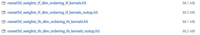
load pre-trained model of resnet50
步骤如下:
- 下载ResNet50不包含全连接层的模型参数到本地(resnet50_weights_tf_dim_ordering_tf_kernels_notop.h5);
- 定义好ResNet50的网络结构;
- 将预训练的模型参数加载到我们所定义的网络结构中;
- 更改全连接层结构,便于对我们的分类任务进行处
- 或者根据需要解冻最后几个block,然后以很低的学习率开始训练。我们只选择最后一个block进行训练,是因为训练样本很少,而ResNet50模型层数很多,全部训练肯定不能训练好,会过拟合。 其次fine-tune时由于是在一个已经训练好的模型上进行的,故权值更新应该是一个小范围的,以免破坏预训练好的特征。
因为使用了预训练模型,参数名称需要和预训练模型一致:
identity层:1
2
3
4
5
6
7
8
9
10
11
12
13
14
15
16
17
18
19
20
21
22
23
24
25
26
27
28
29def identity_block(X, f, filters, stage, block):
# defining name basis
conv_name_base = 'res' + str(stage) + block + '_branch'
bn_name_base = 'bn' + str(stage) + block + '_branch'
# Retrieve Filters
F1, F2, F3 = filters
# Save the input value. You'll need this later to add back to the main path.
X_shortcut = X
# First component of main path
X = Conv2D(filters = F1, kernel_size = (1, 1), strides = (1,1), padding = 'valid', name = conv_name_base + '2a')(X)
X = BatchNormalization(axis = 3, name = bn_name_base + '2a')(X)
X = Activation('relu')(X)
# Second component of main path (≈3 lines)
X = Conv2D(filters= F2, kernel_size=(f,f),strides=(1,1),padding='same',name=conv_name_base + '2b')(X)
X = BatchNormalization(axis=3,name=bn_name_base+'2b')(X)
X = Activation('relu')(X)
# Third component of main path (≈2 lines)
X = Conv2D(filters=F3,kernel_size=(1,1),strides=(1,1),padding='valid',name=conv_name_base+'2c')(X)
X = BatchNormalization(axis=3,name=bn_name_base+'2c')(X)
# Final step: Add shortcut value to main path, and pass it through a RELU activation (≈2 lines)
X = Add()([X, X_shortcut])
X = Activation('relu')(X)
return X
conv层:1
2
3
4
5
6
7
8
9
10
11
12
13
14
15
16
17
18
19
20
21
22
23
24
25
26
27
28
29
30
31
32
33
34
35def convolutional_block(X, f, filters, stage, block, s = 2):
# defining name basis
conv_name_base = 'res' + str(stage) + block + '_branch'
bn_name_base = 'bn' + str(stage) + block + '_branch'
# Retrieve Filters
F1, F2, F3 = filters
# Save the input value
X_shortcut = X
##### MAIN PATH #####
# First component of main path
X = Conv2D(F1, (1, 1), strides = (s,s),padding='valid',name = conv_name_base + '2a')(X)
X = BatchNormalization(axis = 3, name = bn_name_base + '2a')(X)
X = Activation('relu')(X)
# Second component of main path (≈3 lines)
X = Conv2D(F2,(f,f),strides=(1,1),padding='same',name=conv_name_base+'2b')(X)
X = BatchNormalization(axis=3,name=bn_name_base+'2b')(X)
X = Activation('relu')(X)
# Third component of main path (≈2 lines)
X = Conv2D(F3,(1,1),strides=(1,1),padding='valid',name=conv_name_base+'2c')(X)
X = BatchNormalization(axis=3,name=bn_name_base+'2c')(X)
##### SHORTCUT PATH #### (≈2 lines)
X_shortcut = Conv2D(F3,(1,1),strides=(s,s),padding='valid',name=conv_name_base+'1')(X_shortcut)
X_shortcut = BatchNormalization(axis=3,name =bn_name_base+'1')(X_shortcut)
# Final step: Add shortcut value to main path, and pass it through a RELU activation (≈2 lines)
X = Add()([X,X_shortcut])
X = Activation('relu')(X)
return X
resnet50结构:1
2
3
4
5
6
7
8
9
10
11
12
13
14
15
16
17
18
19
20
21
22
23
24
25
26
27
28
29
30
31
32
33
34
35
36
37
38
39
40
41
42
43
44
45
46
47def ResNet50(input_shape = (64, 64, 3), classes = 30):
# Define the input as a tensor with shape input_shape
X_input = Input(input_shape)
# Zero-Padding
X = ZeroPadding2D((3, 3))(X_input)
# Stage 1
X = Conv2D(64, (7, 7), strides = (2, 2), name = 'conv1')(X)
X = BatchNormalization(axis = 3, name = 'bn_conv1')(X)
X = Activation('relu')(X)
X = MaxPooling2D((3, 3), strides=(2, 2))(X)
# Stage 2
X = convolutional_block(X, f = 3, filters = [64, 64, 256], stage = 2, block='a', s = 1)
X = identity_block(X, 3, [64, 64, 256], stage=2, block='b')
X = identity_block(X, 3, [64, 64, 256], stage=2, block='c')
### START CODE HERE ###
# Stage 3 (≈4 lines)
X = convolutional_block(X, f = 3,filters= [128,128,512],stage=3,block='a',s=2)
X = identity_block(X,3,[128,128,512],stage=3,block='b')
X = identity_block(X,3,[128,128,512],stage=3,block='c')
X = identity_block(X,3,[128,128,512],stage=3,block='d')
# Stage 4 (≈6 lines)
X = convolutional_block(X,f=3,filters=[256,256,1024],stage=4,block='a',s=2)
X = identity_block(X,3,[256,256,1024],stage=4,block='b')
X = identity_block(X,3,[256,256,1024],stage=4,block='c')
X = identity_block(X,3,[256,256,1024],stage=4,block='d')
X = identity_block(X,3,[256,256,1024],stage=4,block='e')
X = identity_block(X,3,[256,256,1024],stage=4,block='f')
# Stage 5 (≈3 lines)
X = convolutional_block(X, f = 3,filters= [512,512,2048],stage=5,block='a',s=2)
X = identity_block(X,3,[512,512,2048],stage=5,block='b')
X = identity_block(X,3,[512,512,2048],stage=5,block='c')
# AVGPOOL (≈1 line). Use "X = AveragePooling2D(...)(X)"
X = AveragePooling2D((2,2),strides=(2,2))(X)
# output layer
X = Flatten()(X)
model = Model(inputs = X_input, outputs = X, name='ResNet50')
return model
构建网络并且载入权重:1
2base_model = ResNet50(input_shape=(224,224,3),classes=30)
base_model.load_weights('resnet50_weights_tf_dim_ordering_tf_kernels_notop.h5')
无法载入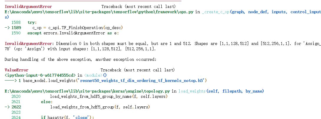
【04/07/2018】
Loading pre-trained model
对于keras:如果新模型和旧模型结构一样,直接调用model.load_weights读取参数就行。如果新模型中的几层和之前模型一样,也通过model.load_weights(‘my_model_weights.h5’, by_name=True)来读取参数, 或者手动对每一层进行参数的赋值,比如x= Dense(100, weights=oldModel.layers[1].get_weights())(x)
修改代码:1
2
3
4
5try:
base_model.load_weights('resnet50_weights_tf_dim_ordering_tf_kernels_notop.h5',by_name=True)
print("load successful")
except:
print("load failed")
载入成功:jupyter notebook
【05~06/07/2018】
construct faster rcnn net
RoiPoolingConv
该函数的作用是对将每一个预选框框定的特征图大小规整到相同大小
什么是ROI呢?
ROI是Region of Interest的简写,指的是在“特征图上的框”;
1)在Fast RCNN中, RoI是指Selective Search完成后得到的“候选框”在特征图上的映射,如下图所示;
2)在Faster RCNN中,候选框是经过RPN产生的,然后再把各个“候选框”映射到特征图上,得到RoIs
创建一个类,这里不同的是它是要继承keras的Layer类1
class RoiPoolingConv(Layer):
定义:
**kwargs:表示的就是形参中按照关键字传值把多余的传值以字典的方式呈现
super:子类调用父类的初始化方法1
2
3
4
5
6
7
8
9
10
11
12
13
14
15
16
17'''ROI pooling layer for 2D inputs.
# Arguments
pool_size: int
Size of pooling region to use. pool_size = 7 will result in a 7x7 region.
num_rois: number of regions of interest to be used
'''
# 第一个是规整后特征图大小 第二个是预选框个数
def __init__(self, pool_size, num_rois, **kwargs):
self.dim_ordering = K.image_dim_ordering()
# print error when kernel not tensorflow or thoean
assert self.dim_ordering in {'tf'}, 'dim_ordering must be in tf'
self.pool_size = pool_size
self.num_rois = num_rois
super(RoiPoolingConv, self).__init__(**kwargs)
得到特征图的输出通道个数:1
2
3def build(self, input_shape):
if self.dim_ordering == 'tf':
self.nb_channels = input_shape[0][3]
定义输出特征图的形状:1
2
3def compute_output_shape(self, input_shape):
if self.dim_ordering == 'tf':
return None, self.num_rois, self.pool_size, self.pool_size, self.nb_channels
遍历提供的所有预选框,将预选宽里的特征图规整到指定大小, 并且加入到output:1
2
3
4
5
6
7
8
9
10
11
12
13
14
15
16
17
18
19
20
21
22
23
24
25
26
27
28
29
30
31
32
33
34
35
36
37
38
39
40def call(self, x, mask=None):
assert(len(x) == 2)
img = x[0]
rois = x[1]
input_shape = K.shape(img)
outputs = []
for roi_idx in range(self.num_rois):
x = rois[0, roi_idx, 0]
y = rois[0, roi_idx, 1]
w = rois[0, roi_idx, 2]
h = rois[0, roi_idx, 3]
row_length = w / float(self.pool_size)
col_length = h / float(self.pool_size)
num_pool_regions = self.pool_size
if self.dim_ordering == 'tf':
x = K.cast(x, 'int32')
y = K.cast(y, 'int32')
w = K.cast(w, 'int32')
h = K.cast(h, 'int32')
# resize porposal of feature map
rs = tf.image.resize_images(img[:, y:y+h, x:x+w, :], (self.pool_size, self.pool_size))
outputs.append(rs)
# 将outputs里面的变量按照第一个维度合在一起【shape:(?, 7, 7, 512)】
final_output = K.concatenate(outputs, axis=0)
final_output = K.reshape(final_output, (1, self.num_rois, self.pool_size, self.pool_size, self.nb_channels))
# 将变量规整到相应的大小【shape:(1, 32, 7, 7, 512)】
final_output = K.permute_dimensions(final_output, (0, 1, 2, 3, 4))
return final_output
输出是batch个vector,其中batch的值等于RoI的个数,vector的大小为channel * w * h;RoI Pooling的过程就是将一个个大小不同的box矩形框,都映射成大小固定(w * h)的矩形框.
TimeDistributed 包装器
FastRcnn在做完ROIpooling后,需要将生产的所有的Roi全部送入分类和回归网络,Keras用的TimeDistributed函数:
Relu激活函数本身就是逐元素计算激活值的,无论进来多少维的tensor都一样,所以不需要使用TimeDistributed。conv2D需要TimeDistributed,是因为一个ROI内的数据计算是互相依赖的,而不同ROI之间又是独立的。
在最后Faster RCNN的结构中进行类别判断和bbox框的回归时,需要对设置的num_rois个感兴趣区域进行回归处理,由于每一个区域的处理是相对独立的,便等价于此时的时间步为num_rois,因此用TimeDistributed来wrap。
改编之前的conv 和 identity层:1
2
3
4
5
6
7
8
9
10
11
12
13
14
15
16
17
18
19
20
21
22
23
24
25
26
27
28def conv_block_td(input_tensor, kernel_size, filters, stage, block, input_shape, strides=(2, 2), trainable=True):
# conv block time distributed
nb_filter1, nb_filter2, nb_filter3 = filters
bn_axis = 3
conv_name_base = 'res' + str(stage) + block + '_branch'
bn_name_base = 'bn' + str(stage) + block + '_branch'
x = TimeDistributed(Convolution2D(nb_filter1, (1, 1), strides=strides, trainable=trainable, kernel_initializer='normal'), input_shape=input_shape, name=conv_name_base + '2a')(input_tensor)
x = TimeDistributed(BatchNormalization(axis=bn_axis), name=bn_name_base + '2a')(x)
x = Activation('relu')(x)
x = TimeDistributed(Convolution2D(nb_filter2, (kernel_size, kernel_size), padding='same', trainable=trainable, kernel_initializer='normal'), name=conv_name_base + '2b')(x)
x = TimeDistributed(BatchNormalization(axis=bn_axis), name=bn_name_base + '2b')(x)
x = Activation('relu')(x)
x = TimeDistributed(Convolution2D(nb_filter3, (1, 1), kernel_initializer='normal'), name=conv_name_base + '2c', trainable=trainable)(x)
x = TimeDistributed(BatchNormalization(axis=bn_axis), name=bn_name_base + '2c')(x)
shortcut = TimeDistributed(Convolution2D(nb_filter3, (1, 1), strides=strides, trainable=trainable, kernel_initializer='normal'), name=conv_name_base + '1')(input_tensor)
shortcut = TimeDistributed(BatchNormalization(axis=bn_axis), name=bn_name_base + '1')(shortcut)
x = Add()([x, shortcut])
x = Activation('relu')(x)
return x
1 | def identity_block_td(input_tensor, kernel_size, filters, stage, block, trainable=True): |
如果将时序信号看作是2D矩阵,则TimeDistributed包装后的Dense就是分别对矩阵的每一行进行全连接。
把resnet50最后一个stage拿出来做分类层:1
2
3
4
5
6
7
8
9
10
11def classifier_layers(x, input_shape, trainable=False):
# Stage 5
x = conv_block_td(x, 3, [512, 512, 2048], stage=5, block='a', input_shape=input_shape, strides=(2, 2), trainable=trainable)
x = identity_block_td(x, 3, [512, 512, 2048], stage=5, block='b', trainable=trainable)
x = identity_block_td(x, 3, [512, 512, 2048], stage=5, block='c', trainable=trainable)
# AVGPOOL
x = TimeDistributed(AveragePooling2D((7, 7)), name='avg_pool')(x)
return x
- RoiPoolingConv:返回的shape为(1, 32, 7, 7, 512)含义是batch_size,预选框的个数,特征图宽,特征图高度,特征图深度
- TimeDistributed:输入至少为3D张量,下标为1的维度将被认为是时间维。即对以一个维度下的变量当作一个完整变量来看待本文是32。你要实现的目的就是对32个预选宽提出的32个图片做出判断。
- out_class的shape:(?, 32, 21); out_regr的shape:(?, 32, 80)
1
2
3
4
5
6
7
8
9
10
11
12
13
14def classifier(base_layers, input_rois, num_rois, nb_classes = 21, trainable=False):
pooling_regions = 14
input_shape = (num_rois,14,14,1024)
out_roi_pool = RoiPoolingConv(pooling_regions, num_rois)([base_layers, input_rois])
out = classifier_layers(out_roi_pool, input_shape=input_shape, trainable=True)
out = TimeDistributed(Flatten())(out)
out_class = TimeDistributed(Dense(nb_classes, activation='softmax', kernel_initializer='zero'), name='dense_class_{}'.format(nb_classes))(out)
# note: no regression target for bg class
out_regr = TimeDistributed(Dense(4 * (nb_classes-1), activation='linear', kernel_initializer='zero'), name='dense_regress_{}'.format(nb_classes))(out)
return [out_class, out_regr]
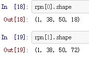
定义RPN网络:
- x_class:每一个锚点属于前景还是背景【注:这里使用的是sigmoid激活函数所以其输出的通道数是num_anchors】
- x_regr:每一个锚点对应的回归梯度
1
2
3
4
5
6
7
8def rpn(base_layers,num_anchors):
x = Convolution2D(512, (3, 3), padding='same', activation='relu', kernel_initializer='normal', name='rpn_conv1')(base_layers)
x_class = Convolution2D(num_anchors, (1, 1), activation='sigmoid', kernel_initializer='uniform', name='rpn_out_class')(x)
x_regr = Convolution2D(num_anchors * 4, (1, 1), activation='linear', kernel_initializer='zero', name='rpn_out_regress')(x)
return [x_class, x_regr, base_layers]
resnet前面部分作为公共层:1
2
3
4
5
6
7
8
9
10
11
12
13
14
15
16
17
18
19
20
21
22
23
24
25
26
27
28
29
30
31
32
33
34
35
36
37
38
39
40
41
42
43
44
45def nn_base(input_tensor=None, trainable=False):
# Determine proper input shape
input_shape = (None, None, 3)
if input_tensor is None:
img_input = Input(shape=input_shape)
else:
if not K.is_keras_tensor(input_tensor):
img_input = Input(tensor=input_tensor, shape=input_shape)
else:
img_input = input_tensor
bn_axis = 3
# Zero-Padding
x = ZeroPadding2D((3, 3))(img_input)
# Stage 1
x = Convolution2D(64, (7, 7), strides=(2, 2), name='conv1', trainable = trainable)(x)
x = BatchNormalization(axis=bn_axis, name='bn_conv1')(x)
x = Activation('relu')(x)
x = MaxPooling2D((3, 3), strides=(2, 2))(x)
# Stage 2
x = conv_block(x, 3, [64, 64, 256], stage=2, block='a', strides=(1, 1), trainable = trainable)
x = identity_block(x, 3, [64, 64, 256], stage=2, block='b', trainable = trainable)
x = identity_block(x, 3, [64, 64, 256], stage=2, block='c', trainable = trainable)
# Stage 3
x = conv_block(x, 3, [128, 128, 512], stage=3, block='a', trainable = trainable)
x = identity_block(x, 3, [128, 128, 512], stage=3, block='b', trainable = trainable)
x = identity_block(x, 3, [128, 128, 512], stage=3, block='c', trainable = trainable)
x = identity_block(x, 3, [128, 128, 512], stage=3, block='d', trainable = trainable)
# Stage 4
x = conv_block(x, 3, [256, 256, 1024], stage=4, block='a', trainable = trainable)
x = identity_block(x, 3, [256, 256, 1024], stage=4, block='b', trainable = trainable)
x = identity_block(x, 3, [256, 256, 1024], stage=4, block='c', trainable = trainable)
x = identity_block(x, 3, [256, 256, 1024], stage=4, block='d', trainable = trainable)
x = identity_block(x, 3, [256, 256, 1024], stage=4, block='e', trainable = trainable)
x = identity_block(x, 3, [256, 256, 1024], stage=4, block='f', trainable = trainable)
return x
搭建网络:1
2
3
4
5
6
7
8
9
10
11
12
13
14
15# define the base network (resnet here)
shared_layers = nn.nn_base(img_input, trainable=True)
# define the RPN, built on the base layers
# 9 types of anchors
num_anchors = len(C.anchor_box_scales) * len(C.anchor_box_ratios)
rpn = nn.rpn(shared_layers, num_anchors)
classifier = nn.classifier(shared_layers, roi_input, C.num_rois, nb_classes=len(classes_count), trainable=True)
model_rpn = Model(img_input, rpn[:2])
model_classifier = Model([img_input, roi_input], classifier)
# this is a model that holds both the RPN and the classifier, used to load/save weights for the models
model_all = Model([img_input, roi_input], rpn[:2] + classifier)
【09/07/2018】
Loss define
由于涉及到分类和回归,所以需要定义一个多任务损失函数(Multi-task Loss Function),包括Softmax Classification Loss和Bounding Box Regression Loss,公式定义如下:
$L({p_{i}},{t_{i}}) = \frac{1}{N_{cls}}\sum_{i}L_{cls}(p_{i},p_{i}^{\ast}) + \lambda\frac{1}{N_{reg}}\sum_{i}L_{reg}(t_{i},t_{i}^{\ast})$
Softmax Classification:
对于RPN网络的分类层(cls),其向量维数为2k = 18,考虑整个特征图conv5-3,则输出大小为W×H×18,正好对应conv5-3上每个点有9个anchors,而每个anchor又有两个score(fg/bg)输出,对于单个anchor训练样本,其实是一个二分类问题。为了便于Softmax分类,需要对分类层执行reshape操作,这也是由底层数据结构决定的。
在上式中,$p_{i}$为样本分类的概率值,$p_{i}^{\ast}$为样本的标定值(label),anchor为正样本时$p_{i}^{\ast}$为1,为负样本时$p_{i}^{\ast}$为0,$L_{cls}$为两种类别的对数损失(log loss)。
Bounding Box Regression:
RPN网络的回归层输出向量的维数为4k = 36,回归参数为每个样本的坐标$[x,y,w,h]$,分别为box的中心位置和宽高,考虑三组参数预测框(predicted box)坐标$[x,y,w,h]$,anchor坐标$[x_{a},y_{a},w_{a},h_{a}]$,ground truth坐标$[x^{\ast},y^{\ast},w^{\ast},h^{\ast}]$,分别计算预测框相对anchor中心位置的偏移量以及宽高的缩放量{$t$},ground truth相对anchor的偏移量和缩放量{$t^{\ast}$}
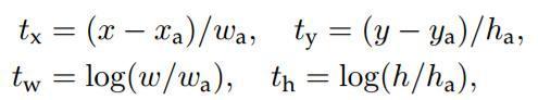
$t_{x}=\frac{(x-x_{a})}{w_{a}}$ , $t_{y}=\frac{(y-y_{a})}{h_{a}}$ , $t_{w}=log(\frac{w}{w_{a}})$ , $t_{h}=log(\frac{h}{h_{a}})$ (1)
$t_{x}^{\ast}=\frac{(x^{\ast}-x_{a})}{w_{a}}$ , $t_{y}^{\ast}=\frac{(y^{\ast}-y_{a})}{h_{a}}$ , $t_{w}^{\ast}=log(\frac{w^{\ast}}{w_{a}})$ , $t_{h}^{\ast}=log(\frac{h^{\ast}}{h_{a}})$ (2)
回归目标就是让{t}尽可能地接近${t^{\ast}}$,所以回归真正预测输出的是${t}$,而训练样本的标定真值为${t^{\ast}}$。得到预测输出${t}$后,通过上式(1)即可反推获取预测框的真实坐标。
在损失函数中,回归损失采用Smooth L1函数:
$$ Smooth_{L1}(x) =\left{
\begin{aligned}
0.5x^{2} \ \ |x| \leqslant 1\
|x| - 0.5 \ \ otherwise
\end{aligned}
\right.
$$
$L_{reg} = Smooth_{L1}(t-t^{\ast})$
Smooth L1损失函数曲线如下图所示,相比于L2损失函数,L1对离群点或异常值不敏感,可控制梯度的量级使训练更易收敛。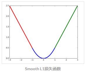
在损失函数中,$p_{i}^{\ast}L_{reg}$这一项表示只有目标anchor$(p_{i}^{\ast}=1)$才有回归损失,其他anchor不参与计算。这里需要注意的是,当样本bbox和ground truth比较接近时(IoU大于某一阈值),可以认为上式的坐标变换是一种线性变换,因此可将样本用于训练线性回归模型,否则当bbox与ground truth离得较远时,就是非线性问题,用线性回归建模显然不合理,会导致模型不work。分类层(cls)和回归层(reg)的输出分别为{p}和{t},两项损失函数分别由$N_{cls}$和$N_{reg}$以及一个平衡权重λ归一化。
【10/07/2018】
loss code
generator to iteror, using next() to loop1
yield np.copy(x_img), [np.copy(y_rpn_cls), np.copy(y_rpn_regr)], img_data_aug
Rpn calculation:1
img,rpn,img_aug = next(data_gen_train)
连续两个def 是装饰器,
装饰器其实也就是一个函数,一个用来包装函数的函数,返回一个修改之后的函数对象。经常被用于有切面需求的场景,较为经典的有插入日志、
性能测试、事务处理等。装饰器是解决这类问题的绝佳设计,有了装饰器,我们就可以抽离出大量函数中与函数功能本身无关的雷同代码并继续重用。概括的讲,装
饰器的作用就是为已经存在的对象添加额外的功能。
根据:$L$ 的 cls 部分
$L({p_{i}},{t_{i}}) = \frac{1}{N_{cls}}\sum_{i}L_{cls}(p_{i},p_{i}^{\ast})$
在上式中,$p_{i}$为样本分类的概率值,$p_{i}^{\ast}$为样本的标定值(label),anchor为正样本时$p_{i}^{\ast}$为1,为负样本时$p_{i}^{\ast}$为0,$L_{cls}$为两种类别的对数损失(log loss)。
因此, 定义 rpn loss cls:1
2
3
4
5
6def rpn_loss_cls(num_anchors):
def rpn_loss_cls_fixed_num(y_true, y_pred):
# binary_crossentropy -> logloss
# epsilon to increase robustness
return lambda_rpn_class * K.sum(y_true[:, :, :, :num_anchors] * K.binary_crossentropy(y_pred[:, :, :, :], y_true[:, :, :, num_anchors:])) / K.sum(epsilon + y_true[:, :, :, :num_anchors])
return rpn_loss_cls_fixed_num
根据$L$ 的 reg 部分
$L({p_{i}},{t_{i}}) = \lambda\frac{1}{N_{reg}}\sum_{i}L_{reg}(t_{i},t_{i}^{\ast})$
在损失函数中,回归损失采用Smooth L1函数:
$$ Smooth_{L1}(x) =\left{
\begin{aligned}
0.5x^{2} \ \ |x| \leqslant 1\
|x| - 0.5 \ \ otherwise
\end{aligned}
\right.
$$
$L_{reg} = Smooth_{L1}(t-t^{\ast})$
因此, 定义 rpn loss reg:1
2
3
4
5
6
7
8
9
10
11
12
13def rpn_loss_regr(num_anchors):
def rpn_loss_regr_fixed_num(y_true, y_pred):
# difference of ture value and predicted value
x = y_true[:, :, :, 4 * num_anchors:] - y_pred
# absulote value of difference
x_abs = K.abs(x)
# if absulote value less than 1, x_bool == 1, else x_bool = 0
x_bool = K.cast(K.less_equal(x_abs, 1.0), tf.float32)
return lambda_rpn_regr * K.sum(y_true[:, :, :, :4 * num_anchors] * (x_bool * (0.5 * x * x) + (1 - x_bool) * (x_abs - 0.5))) / K.sum(epsilon + y_true[:, :, :, :4 * num_anchors])
return rpn_loss_regr_fixed_num
对class的loss来说用一样的方程,但是class_loss_cls是无差别求loss【这个可以用K.mean,是因为其是无差别的求loss】,不用管是否可用1
2
3
4
5
6
7
8
9
10
11def class_loss_regr(num_classes):
def class_loss_regr_fixed_num(y_true, y_pred):
x = y_true[:, :, 4*num_classes:] - y_pred
x_abs = K.abs(x)
x_bool = K.cast(K.less_equal(x_abs, 1.0), 'float32')
return lambda_cls_regr * K.sum(y_true[:, :, :4*num_classes] * (x_bool * (0.5 * x * x) + (1 - x_bool) * (x_abs - 0.5))) / K.sum(epsilon + y_true[:, :, :4*num_classes])
return class_loss_regr_fixed_num
def class_loss_cls(y_true, y_pred):
return lambda_cls_class * K.mean(categorical_crossentropy(y_true[0, :, :], y_pred[0, :, :]))
【11/07/2018】
Iridis
High Performance Computing (HPC)

Iridis 5 specifications
- #251 in hte world(Based on July 2018 TOPP500 list) with $R_{peak}\sim1305.6\ TFlops/s$
- 464 2.0 GHz nodes with 40 cores per node, 192 GB memeory
- 10 nodes with 4xGTX1080TI GPUs, 28 cores(hyper-threaded), 128 GB memeory
- 10 nodes with 2xVolta Tesia GPUs, same as thandard compute
- 2.2 PB disk with paraller file system (>12GB\s)
- £5M Project delivered by OCF/IBM
create my own conda envieroment
Fllowing instroduction before
Slurm command
| Command | Definition |
|---|---|
| sbatch | Submits job scripts into system for execution (queued) |
| scancel | Cancels a job |
| scontrol | Used to display Slurm state, several options only available to root |
| sinfo | Display state of partitions and nodes |
| squeue | Display state of jobs |
| salloc | Submit a job for execution, or initiate job in real time |
Bash script1
2
3
4
5
6
7
8
9
10
11
12
13
14
#SBATCH -J faster_rcnn
#SBATCH -o train_7.out
#SBATCH --ntasks=28
#SBATCH --nodes=1
#SBATCH --ntasks-per-node=8
#SBATCH --time=00:05:00
#SBATCH --gres=gpu:1
#SBATCH -p lyceum
module load conda
module load cuda
source activate project
python test_frcnn.py
【12~13/07/2018】
change plan
因为faster r-cnn的搭建过程比想象中复杂,在咨询老师的意见以后,决定砍掉capsule的测试,专心faster-rcnn并且找到一些fine turn的方法。
1)基础特征提取网络
ResNet,IncRes V2,ResNeXt 都是显著超越 VGG 的特征网络,当然网络的改进带来的是计算量的增加。
2)RPN
通过更准确地 RPN 方法,减少 Proposal 个数,提高准确度。
3)改进分类回归层
分类回归层的改进,包括 通过多层来提取特征 和 判别。
@改进1:ION
论文:Inside outside net: Detecting objects in context with skip pooling and recurrent neural networks
提出了两个方面的贡献:
1)Inside Net
所谓 Inside 是指在 ROI 区域之内,通过连接不同 Scale 下的 Feature Map,实现多尺度特征融合。
这里采用的是 Skip-Pooling,从 conv3-4-5-context 分别提取特征,后面会讲到。
多尺度特征 能够提升对小目标的检测精度。
2)Outside Net
所谓 Outside 是指 ROI 区域之外,也就是目标周围的 上下文(Contextual)信息。
作者通过添加了两个 RNN 层(修改后的 IRNN)实现上下文特征提取。
上下文信息 对于目标遮挡有比较好的适应。
@改进2:多尺度之 HyperNet
论文:Hypernet: Towards accurate region proposal generation and joint object detection
基于 Region Proposal 的方法,通过多尺度的特征提取来提高对小目标的检测能力,来看网络框图: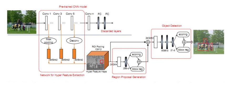
分为 三个主要特征 来介绍(对应上面网络拓扑图的 三个红色框):
1)Hyper Feature Extraction (特征提取)
多尺度特征提取是本文的核心点,作者的方法稍微有所不同,他是以中间的 Feature 尺度为参考,前面的层通过 Max Pooling 到对应大小,后面的层则是通过 反卷积(Deconv)进行放大。
多尺度 Feature ConCat 的时候,作者使用了 LRN进行归一化(类似于 ION 的 L2 Norm)。
2)Region Proposal Generation(建议框生成)
作者设计了一个轻量级的 ConvNet,与 RPN 的区别不大(为写论文强创新)。
一个 ROI Pooling层,一个 Conv 层,还有一个 FC 层。每个 Position 通过 ROI Pooling 得到一个 13*13 的 bin,通过 Conv(3*3*4)层得到一个 13*13*4 的 Cube,再通过 FC 层得到一个 256d 的向量。
后面的 Score+ BBox_Reg 与 Faster并无区别,用于目标得分 和 Location OffSet。
考虑到建议框的 Overlap,作者用了 Greedy NMS 去重,文中将 IOU参考设为 0.7,每个 Image 保留 1k 个 Region,并选择其中 Top-200 做 Detetcion。
通过对比,要优于基于 Edge Box 重排序的 Deep Box,从多尺度上考虑比 Deep Proposal 效果更好。
3)Object Detection(目标检测)
与 Fast RCNN基本一致,在原来的检测网络基础上做了两点改进:
a)在 FC 层之前添加了一个 卷积层(3363),对特征有效降维;
b)将 DropOut 从 0.5 降到 0.25;
另外,与 Proposal一样采用了 NMS 进行 Box抑制,但由于之前已经做了,这一步的意义不大。
@改进3:多尺度之 MSCNN
论文:A Unified Multi-scale Deep Convolutional Neural Network for Fast Object Detection
a)原图缩放,多个Scale的原图对应不同Scale的Feature;
该方法计算多次Scale,每个Scale提取一次Feature,计算量巨大。
b)一幅输入图像对应多个分类器;
不需要重复提取特征图,但对分类器要求很高,一般很难得到理想的结果。
c)原图缩放,少量Scale原图->少量特征图->多个Model模板;
相当于对 a)和 b)的 Trade-Off。
d)原图缩放,少量Scale原图->少量特征图->特征图插值->1个Model;
e)RCNN方法,Proposal直接给到CNN;
和 a)全图计算不同,只针对Patch计算。
f)RPN方法,特征图是通过CNN卷积层得到;
和 b)类似,不过采用的是同尺度的不同模板,容易导致尺度不一致问题。
g)上套路,提出我们自己的方法,多尺度特征图;
每个尺度特征图对应一个 输出模板,每个尺度cover一个目标尺寸范围。
NMS和soft-nms算法
Repulsion loss:遮挡下的行人检测 加入overlapping 与不同的 loss
融合以上两个到faster rcnn中
【16~20/07/2018】
旅行
【23/07/2018】
fix boxes location by regrident
使用regr对anchor所确定的框进行修正
1 | """ fix boxes with grident |
$t_{x}=\frac{(x-x_{a})}{w_{a}}$ , $t_{y}=\frac{(y-y_{a})}{h_{a}}$ , $t_{w}=log(\frac{w}{w_{a}})$ , $t_{h}=log(\frac{h}{h_{a}})$ (1)
$t_{x}^{\ast}=\frac{(x^{\ast}-x_{a})}{w_{a}}$ , $t_{y}^{\ast}=\frac{(y^{\ast}-y_{a})}{h_{a}}$ , $t_{w}^{\ast}=log(\frac{w^{\ast}}{w_{a}})$ , $t_{h}^{\ast}=log(\frac{h^{\ast}}{h_{a}})$ (2)
回归目标就是让{t}尽可能地接近${t^{\ast}}$,所以回归真正预测输出的是${t}$,而训练样本的标定真值为${t^{\ast}}$。得到预测输出${t}$后,通过上式(1)即可反推获取预测框的真实坐标。
过程:1
2
3
4
5
6
7
8
9
10
11
12
13
14
15
16
17
18
19
20
21
22
23
24 # centre cordinate
cx = x + w/2.
cy = y + h/2.
# fixed centre cordinate
cx1 = tx * w + cx
cy1 = ty * h + cy
# fixed wdith and height
w1 = np.exp(tw.astype(np.float64)) * w
h1 = np.exp(th.astype(np.float64)) * h
# fixed left top corner's cordinate
x1 = cx1 - w1/2.
y1 = cy1 - h1/2.
# apporximate
x1 = np.round(x1)
y1 = np.round(y1)
w1 = np.round(w1)
h1 = np.round(h1)
return np.stack([x1, y1, w1, h1])
except Exception as e:
print(e)
return X
NMS no max suppression
该函数的作用是从所给定的所有预选框中选择指定个数最合理的边框。
定义:1
2
3
4
5
6
7
8
9
10
11
12""" NMS , delete overlapping box
@param boxes: (n,4) box and coresspoding cordinates
@param probs: (n,) box adn coresspding possibility
@param overlap_thresh: treshold of delet box overlapping
@param max_boxes: maximum keeping number of boxes
@return: boxes: boxes cordinates(x1,y1,x2,y2)
@return: probs: coresspoding possibility
"""
def non_max_suppression_fast(boxes, probs, overlap_thresh=0.9, max_boxes=300):
1 | if len(boxes) == 0: |
对输入的数据进行确认
不能为空
左上角的坐标小于右下角
数据类型的转换1
2
3
4
5
6
7
8# initialize the list of picked indexes
pick = []
# calculate the areas
area = (x2 - x1) * (y2 - y1)
# sort the bounding boxes
idxs = np.argsort(probs)
pick(拾取)用来存放边框序号
计算框的面积
probs按照概率从小到大排序1
2
3
4
5
6while len(idxs) > 0:
# grab the last index in the indexes list and add the
# index value to the list of picked indexes
last = len(idxs) - 1
i = idxs[last]
pick.append(i)
接下来就是按照概率从大到小取出框,且框的重合度不可以高于overlap_thresh。代码的思路是这样的:
每一次取概率最大的框(即idxs最后一个)
删除掉剩下的框中重和度高于overlap_thresh的框
直到取满max_boxes为止1
2
3
4
5
6
7
8
9
10
11# find the intersection
xx1_int = np.maximum(x1[i], x1[idxs[:last]])
yy1_int = np.maximum(y1[i], y1[idxs[:last]])
xx2_int = np.minimum(x2[i], x2[idxs[:last]])
yy2_int = np.minimum(y2[i], y2[idxs[:last]])
ww_int = np.maximum(0, xx2_int - xx1_int)
hh_int = np.maximum(0, yy2_int - yy1_int)
area_int = ww_int * hh_int
取出idxs队列中最大概率框的序号,将其添加到pick中1
2
3
4
5
6
7
8# find the union
area_union = area[i] + area[idxs[:last]] - area_int
# compute the ratio of overlap
overlap = area_int/(area_union + 1e-6)
# delete all indexes from the index list that have
idxs = np.delete(idxs, np.concatenate(([last],np.where(overlap > overlap_thresh)[0])))
计算取出来的框与剩下来的框区域的交集1
2if len(pick) >= max_boxes:
break
计算重叠率,然后删除掉重叠率较高的位置[np.concatest],是因为最后一个位置你已经用过了,就得将其从队列中删掉
当取足max_boxes框,停止循环1
2
3boxes = boxes[pick].astype("int")
probs = probs[pick]
return boxes, probs
返回pick内存取的边框和对应的概率
【24/07/2018】
rpn to porposal fixed
该函数的作用是将rpn网络的预测结果转化到一个个预选框
函数流程:
遍历anchor_size,在遍历anchor_ratio
得到框的长宽在原图上的映射
得到相应尺寸的框对应的回归梯度,将深度都放到第一个维度
注1:regr_layer[0, :, :, 4 * curr_layer:4 * curr_layer + 4]当某一个维度的取值为一个值时,那么新的变量就会减小一个维度
注2:curr_layer代表的是特定长度和比例的框所代表的编号
得到anchor对应的(x,y,w,h)
使用regr对anchor所确定的框进行修正
对修正后的边框一些不合理的地方进行矫正。
如,边框回归后的左上角和右下角的点不能超过图片外,框的宽高不可以小于0
注:得到框的形式是(x1,y1,x2,y2)
得到all_boxes形状是(n,4),和每一个框对应的概率all_probs形状是(n,)
删除掉一些不合理的点,即右下角的点值要小于左上角的点值
注:np.where() 返回位置信息,这也是删除不符合要求点的一种方法
np.delete(all_boxes, idxs, 0)最后一个参数是在哪一个维度删除
最后是根据要求选取指定个数的合理预选框。这一步是重要的,因为每一个点可以有9个预选框,而又拥有很多点,一张图片可能会有几万个预选框。而经过这一步预选迅速下降到几百个。1
2
3
4
5
6
7
8
9
10
11
12
13
14
15
16
17
18
19
20
21
22
23
24
25
26
27
28
29
30
31
32
33
34
35
36
37
38
39
40
41
42
43
44
45
46
47
48
49
50
51
52
53
54
55
56
57
58
59
60
61
62
63
64
65
66
67
68
69
70
71
72
73
74
75
76
77
78
79
80
81
82
83
84
85
86
87
88
89
90
91
92
93
94
95
96
97
98
99
100""" rpn to porposal
@param rpn_layer: porposal's coresspoding possibiliy, whether item exciseted
@param regr_layer: porposal's coresspoding regrident
@param C: Configuration
@param dim_ordering: Dimensional organization
@param use_regr=True: wether use regurident to fix proposal
@param max_boxes=300: max boxes after apply this function
@param overlap_thresh=0.9: threshold of overlapping
@param C: Configuration
@return: max_boxes proposal with format (x1,y1,x2,y2)
"""
def rpn_to_roi(rpn_layer, regr_layer, C, dim_ordering, use_regr=True, max_boxes=300,overlap_thresh=0.9):
# std_scaling default 4
regr_layer = regr_layer / C.std_scaling
anchor_sizes = C.anchor_box_scales
anchor_ratios = C.anchor_box_ratios
assert rpn_layer.shape[0] == 1
# obtain img's width and height's matrix
(rows, cols) = rpn_layer.shape[1:3]
curr_layer = 0
A = np.zeros((4, rpn_layer.shape[1], rpn_layer.shape[2], rpn_layer.shape[3]))
# anchor size is [128, 256, 512]
for anchor_size in anchor_sizes:
# anchor ratio is [1,2,1]
for anchor_ratio in anchor_ratios:
# rpn_stride = 16
# obatin anchor's weidth and height on feature map
anchor_x = (anchor_size * anchor_ratio[0])/C.rpn_stride
anchor_y = (anchor_size * anchor_ratio[1])/C.rpn_stride
# obtain current regrident
# when one dimentional obtain a value, the new varirant will decrease one dimenttion
regr = regr_layer[0, :, :, 4 * curr_layer:4 * curr_layer + 4]
# put depth to first bacause tensorflow as backend
regr = np.transpose(regr, (2, 0, 1))
# The rows of the output array X are copies of the vector x; columns of the output array Y are copies of the vector y
# each cordinartes of matrix cls and rows
X, Y = np.meshgrid(np.arange(cols),np. arange(rows))
# obtain anchors's (x,y,w,h)
A[0, :, :, curr_layer] = X - anchor_x/2
A[1, :, :, curr_layer] = Y - anchor_y/2
A[2, :, :, curr_layer] = anchor_x
A[3, :, :, curr_layer] = anchor_y
# fix boxes with grident
if use_regr:
# fixed corinates of box
A[:, :, :, curr_layer] = apply_regr_np(A[:, :, :, curr_layer], regr)
# fix unreasonable cordinates
# np.maximum(1,[]) will set the value less than 1 in [] to 1
# box's width and height can't less than 0
A[2, :, :, curr_layer] = np.maximum(1, A[2, :, :, curr_layer])
A[3, :, :, curr_layer] = np.maximum(1, A[3, :, :, curr_layer])
# fixed right bottom cordinates
A[2, :, :, curr_layer] += A[0, :, :, curr_layer]
A[3, :, :, curr_layer] += A[1, :, :, curr_layer]
# left top corner cordinates can't out image
A[0, :, :, curr_layer] = np.maximum(0, A[0, :, :, curr_layer])
A[1, :, :, curr_layer] = np.maximum(0, A[1, :, :, curr_layer])
# right bottom corner cordinates can't out img
A[2, :, :, curr_layer] = np.minimum(cols-1, A[2, :, :, curr_layer])
A[3, :, :, curr_layer] = np.minimum(rows-1, A[3, :, :, curr_layer])
# next layer
curr_layer += 1
# obtain (n,4) object and coresspoding cordinate
all_boxes = np.reshape(A.transpose((0, 3, 1,2)), (4, -1)).transpose((1, 0))
# obtain(n,) object and creoespdoing possibility
all_probs = rpn_layer.transpose((0, 3, 1, 2)).reshape((-1))
# cordinates of left top and right bottom of box
x1 = all_boxes[:, 0]
y1 = all_boxes[:, 1]
x2 = all_boxes[:, 2]
y2 = all_boxes[:, 3]
# find where right cordinate bigger than left cordinate
idxs = np.where((x1 - x2 >= 0) | (y1 - y2 >= 0))
# delete thoese point at 0 dimentional -> all boxes
all_boxes = np.delete(all_boxes, idxs, 0)
all_probs = np.delete(all_probs, idxs, 0)
# apply NMS to reduce overlapping boxes
result = non_max_suppression_fast(all_boxes, all_probs, overlap_thresh=overlap_thresh, max_boxes=max_boxes)[0]
return result
【25/07/2018】
generate classifier’s trainning data
该函数的作用是生成classifier网络训练的数据,需要注意的是它对提供的预选框还会做一次选择就是将容易判断的背景删除
代码流程:
得到图片的基本信息,并将图片的最短边规整到相应的长度。并将bboxes的长度做相应的变化
遍历所有的预选框R, 将每一个预选框与所有的bboxes求交并比,记录最大交并比。用来确定该预选框的类别。
对最佳的交并比作不同的判断:
当最佳交并比小于最小的阈值时,放弃概框。因为,交并比太低就说明是很好判断的背景没必要训练。当大于最小阈值时,则保留相关的边框信息
当在最小和最大之间,就认为是背景。有必要进行训练。
大于最大阈值时认为是物体,计算其边框回归梯度
得到该类别对应的数字
将该数字对应的地方置为1【one-hot】
将该类别加入到y_class_num
coords是用来存储边框回归梯度的,labels来决定是否要加入计算loss中1
2
3
4
5
6
7
8class_num = 2
class_label = 10 * [0]
print(class_label)
class_label[class_num] = 1
print(class_label)
输出:
[0, 0, 0, 0, 0, 0, 0, 0, 0, 0]
[0, 0, 1, 0, 0, 0, 0, 0, 0, 0]
如果不是背景的话,计算相应的回归梯度
返回数据
1 | """ generate classifier training data |
【26~27/07/2018】
model parameters
1 | # rpn optimizer |
Training process
函数流程:
训练rpn网络并且进行预测:
训练RPN网络,X是图片、Y是对应类别和回归梯度【注:并不是所有的点都参与训练,只有符合条件的点才参与训练】
根据rpn网络的预测结果得到classifier网络的训练数据:
将预测结果转化为预选框
计算宽属于哪一类,回归梯度是多少
如果没有有效的预选框则结束本次循环
得到正负样本在的位置【Y1[0, :, -1]:0指定batch的位置,:指所有框,-1指最后一个维度即背景类】
neg_samples = neg_samples[0]:这样做的原因是将其变为一维的数组
下面这一步是选择C.num_rois个数的框,送入classifier网络进行训练。思路是:当C.num_rois大于1的时候正负样本尽量取到各一半,小于1的时候正负样本随机取一个。需要注意的是我们这是拿到的是正负样本在的位置而不是正负样本本身,这也是随机抽取的一般方法
训练classifier网络:
打印Loss和accury
如果网络有两个不同的输出,那么第一个是和损失接下来是分损失【loss_class[3]:代表是准确率在定义网络的时候定义了】1
2classifer网络的loss输出:
[1.4640709, 1.0986123, 0.36545864, 0.15625]
还有就是这些loss都是list数据类型,所以要把它倒腾到numpy数据中
当结束一轮的epoch时,只有当这轮epoch的loss小于最优的时候才会存储这轮的训练数据。并结束这轮epoch进入下一轮epoch.
1 | # Training Process |
【30/07/2018】
Running at GPU enviorment
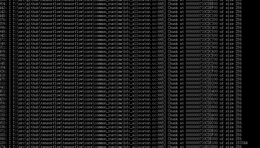
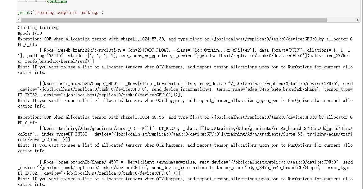
Meet error in GPU version tensorflow
No enough memory.
Try to Running at Irius:
Setting 3 differnet configration:
at Prjoect1 file:
set epoch_length to number of training img1
2epoch_length = 11540
num_epochs = 100
Apply img enhance function1
2
3C.use_horizontal_flips = True
C.use_vertical_flips = True
C.rot_90 = True
at Prjoect file:
set epoch_length to 1000, increase epoch1
2epoch_length = 1000
num_epochs = 2000
Apply img enhance and class balance function1
2
3
4C.use_horizontal_flips = True
C.use_vertical_flips = True
C.rot_90 = True
C.balanced_classes = True
at Prjoect3 file:
set epoch_length to 1000, increase epoch1
2epoch_length = 1000
num_epochs = 2000
Apply img enhance1
2
3C.use_horizontal_flips = True
C.use_vertical_flips = True
C.rot_90 = True
check irdius work
1 | myqueue |

1 | ssh pink59 |
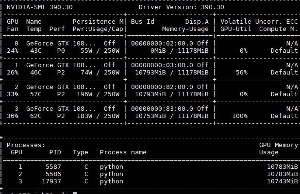
【31/07/2018】
obtain trained model and log file
因为 Iriuds 的GPU使用时长限制最高为24小时,因此,需要在下一次开始前载入上一次训练的模型。
每次训练的粗略结果更新在LogBook最前面.
plot rpn and classfier loss
获取日志中每个小epoch的rpn_cls, rpn_regr, detc_cls, detc_regr
遍历日志,用正则匹配出相应的数值添加到List中:1
2
3
4
5
6
7
8
9
10
11
12
13
14
15
16
17
18
19
20
21
22
23
24
25
26
27
28
29
30
31
32
33
34
35
36
37
38def obtain_each_batch(filename):
n = 0
rpn_cls = []
rpn_regr = []
detector_cls = []
detector_regr = []
f = open(filename,'r',buffering=-1)
lines = f.readlines()
for line in lines:
n = n + 1
match = re.match(r'.* - rpn_cls: (.*) - rpn_regr: .*', line, re.M|re.I)
if match is None:
continue
else:
rpn_cls.append(float(match.group(1)))
match = re.match(r'.* - rpn_regr: (.*) - detector_cls: .*', line, re.M|re.I)
if match is None:
continue
else:
rpn_regr.append(float(match.group(1)))
match = re.match(r'.* - detector_cls: (.*) - detector_regr: .*', line, re.M|re.I)
if match is None:
continue
else:
detector_cls.append(float(match.group(1)))
match = re.match(r'.* - detector_regr: (.*)\n', line, re.M|re.I)
if match is None:
continue
else:
det_regr = match.group(1)[0:6]
detector_regr.append(float(det_regr))
f.close()
print(n)
return rpn_cls, rpn_regr, detector_cls, detector_regr
每个epoch都会计算accury, loss of rpn cls, loss of rpn regr, loss of detc cls, loss of detc regr
遍历日志找到相应的数值添加到list中:1
2
3
4
5
6
7
8
9
10
11
12
13
14
15
16
17
18
19
20
21
22
23
24
25
26
27
28
29
30
31
32
33
34
35def obtain_batch(filename):
n = 0
accuracy = []
loss_rpn_cls = []
loss_rpn_regr = []
loss_detc_cls = []
loss_detc_regr = []
f = open(filename,'r',buffering=-1)
lines = f.readlines()
for line in lines:
n = n + 1
if 'Classifier accuracy for bounding boxes from RPN' in line:
result = re.findall(r"\d+\.?\d*",line)
accuracy.append(float(result[0]))
if 'Loss RPN classifier' in line:
result = re.findall(r"\d+\.?\d*",line)
loss_rpn_cls.append(float(result[0]))
if 'Loss RPN regression' in line:
result = re.findall(r"\d+\.?\d*",line)
loss_rpn_regr.append(float(result[0]))
if 'Loss Detector classifier' in line:
result = re.findall(r"\d+\.?\d*",line)
loss_detc_cls.append(float(result[0]))
if 'Loss Detector regression' in line:
result = re.findall(r"\d+\.?\d*",line)
loss_detc_regr.append(float(result[0]))
f.close()
print(n)
return accuracy, loss_rpn_cls, loss_rpn_regr, loss_detc_cls, loss_detc_regr
plot epoch loss and accury
1 | filename = r'F:\desktop\新建文件夹\1000-no_balance\train1.out' |
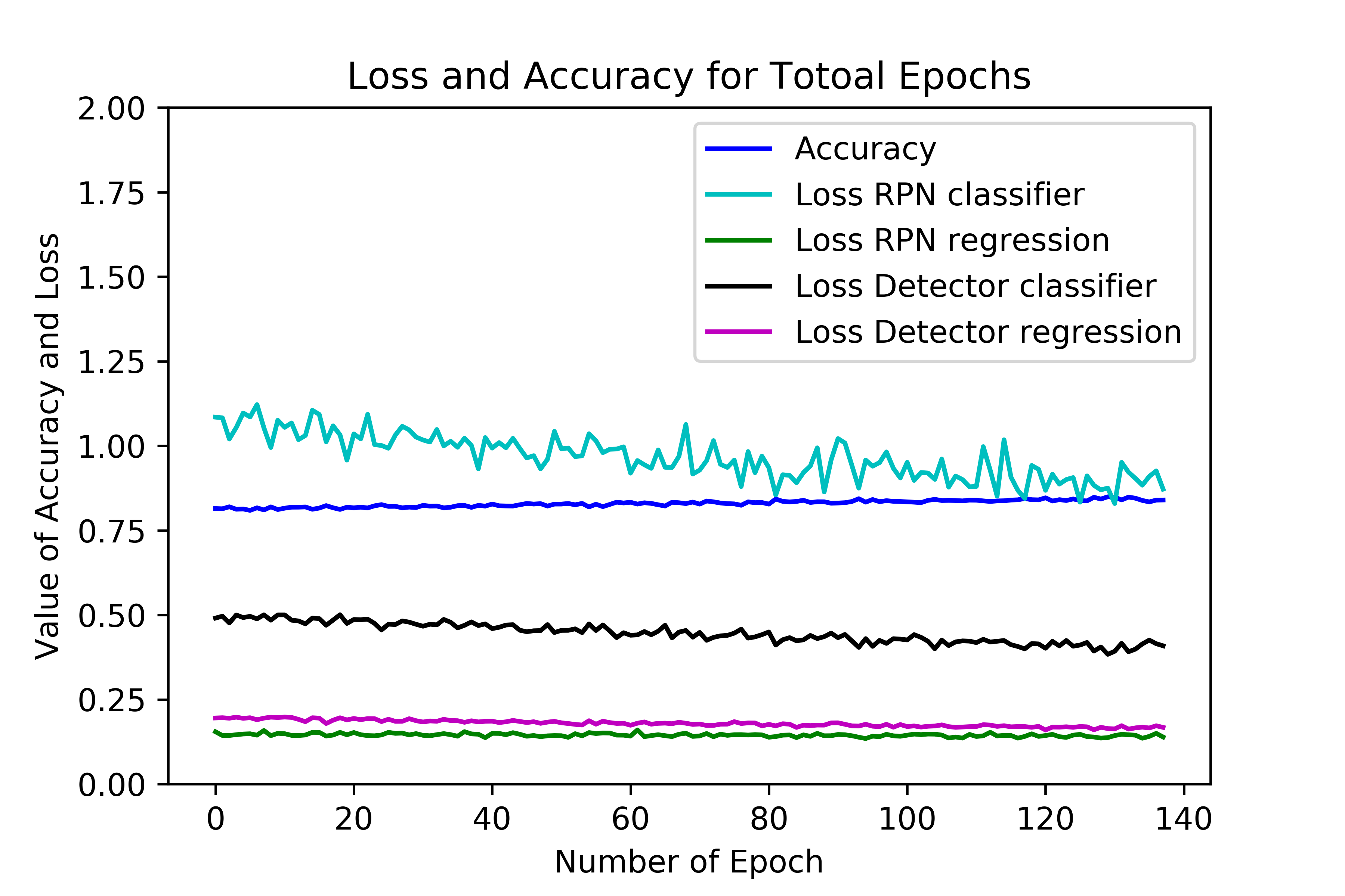
1 | filename = r'F:\desktop\新建文件夹\1000-no_balance\train1.out' |
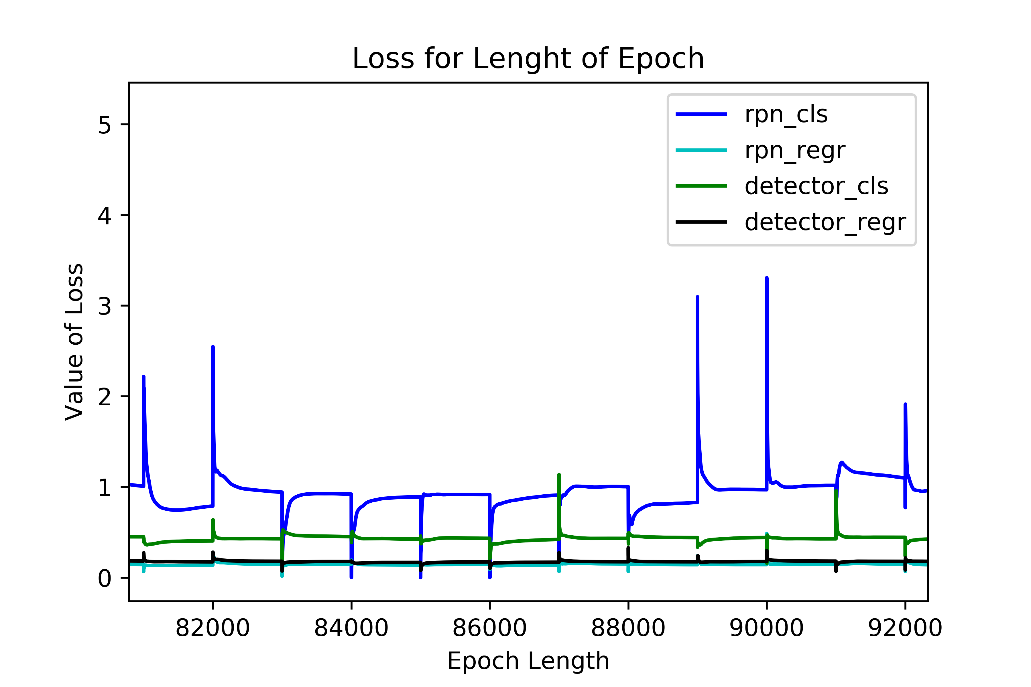
August
【01~02/08/2018】
test network
首先是搭建网络,用于train部分相同的设置搭建
不过在这里图像增强就设置为关闭了
构建rpn输出1
2
3shared_layers = nn.nn_base(img_input, trainable=True)
num_anchors = len(C.anchor_box_scales)*len(C.anchor_box_ratios)
rpn_layers = nn.rpn(shared_layers,num_anchors)
构建classifier输出,参数分别是:特征层输出,预选框,探测框的数目,多少个类,是否可训练1
classifier = nn.classifier(feature_map_input, roi_input, C.num_rois,nb_classes=len(class_mapping), trainable=True)
载入训练好的权重:1
2
3
4
5
6
7C.model_path = 'gpu_resnet50_weights.h5'
try:
print('Loading weights from {}'.format(C.model_path))
model_rpn.load_weights(C.model_path, by_name=True)
model_classifier.load_weights(C.model_path, by_name=True)
except:
print('can not load')
读取需要检测的图片: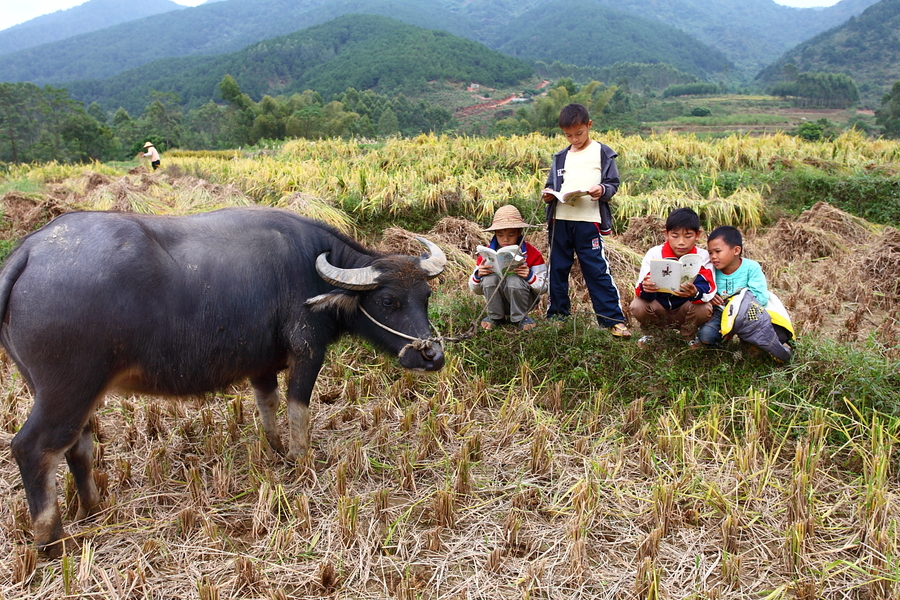
将图片规整到制定的大小
将图片缩放到规定的大小
首先从配置文件夹中得到最小边的大小
得到图片的高度和宽度
根据高度和宽度谁大谁小,确定规整后图片的高宽
将图片缩放到指定的大小,用的是立方插值。返回的缩放后的图片img和相应的缩放的比例。1
2
3
4
5
6
7
8
9def format_img_size(img, C):
(height,width,_) = img.shape
if width <= height:
ratio = C.im_size/width
else:
ratio = C.im_size/height
new_width, new_height = image_processing.get_new_img_size(width,height, C.im_size)
img = cv2.resize(img, (new_width, new_height), interpolation=cv2.INTER_CUBIC)
return img, ratio对图片每一个通道的像素值做规整
将图片的BGR变成RGB,因为网上训练好的RESNET图片都是以此训练的
将图片数据类型转换为np.float32,并减去每一个通道的均值,理由同上
图片的像素值除一个缩放因子,此处为1
将图片的深度变到第一个位置
给图片增加一个维度1
2
3
4
5
6
7
8
9
10
11def format_img_channels(img, C):
""" formats the image channels based on config """
img = img[:, :, (2, 1, 0)]
img = img.astype(np.float32)
img[:, :, 0] -= C.img_channel_mean[0]
img[:, :, 1] -= C.img_channel_mean[1]
img[:, :, 2] -= C.img_channel_mean[2]
img /= C.img_scaling_factor
img = np.transpose(img, (2, 0, 1))
img = np.expand_dims(img, axis=0)
return img
如果用的是tensorflow内核,需要将图片的深度变换到最后一位。
进行区域预测
Y1:anchor包含物体的概率
Y2:每一个anchor对应的回归梯度
F:卷积后的特征图,接下来会有用
1 | [Y1, Y2, F] = model_rpn.predict(X) |
获得rpn预测的结果以及对应的回归梯度,这一步就是对图片上隔16个像素的每个anchor进行rpn计算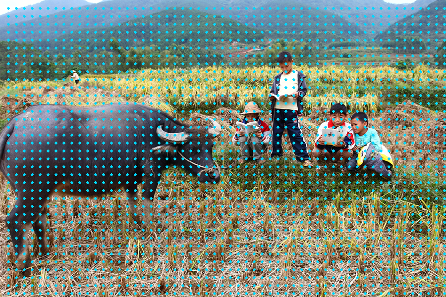
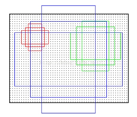
根据rpn预测的结果,得到预选框:
这里会返回300个预选框以及它们对应的坐标(x1,y1,x2,y2)1
2# transform predicted rpn to cordinates of boxes
R = rpn_to_boxes.rpn_to_roi(Y1, Y2, C, K.image_dim_ordering(), use_regr=True, overlap_thresh=0.7)
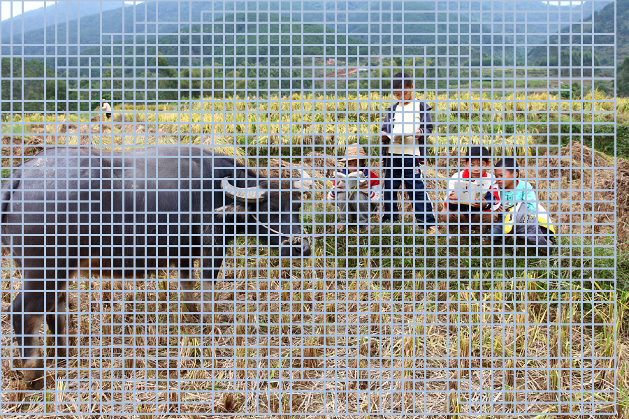
将预选框的坐标由(x1,y1,x2,y2) 改到 (x,y,w,h)1
2R[:, 2] -= R[:, 0]
R[:, 3] -= R[:, 1]
遍历所有的预选框
需要注意的是每一次遍历预选框的个数为C.num_rois
每一次遍历32个预选框,那么总共需要300/32, 10批次
取出32个预选框,并增加一个维度【注:当不满一个32,其自动只取到最后一个】
当预选框被取空的时候,停止循环
当最后一次去不足32个预选框时,补第一个框使其达到32个。1
2
3
4
5
6
7
8
9
10
11
12
13
14
15
16
17
18
19
20# divided 32 bboxes as one group
for jk in range(R.shape[0]//C.num_rois + 1):
# pick num_rios(32) bboxes one time, only pick to last bboxes in last group
ROIs = np.expand_dims(R[C.num_rois*jk:C.num_rois*(jk+1), :], axis=0)
#print(ROIs.shape)
# no proposals, out iter
if ROIs.shape[1] == 0:
break
# when last time can't obtain num_rios(32) bboxes, adding bboxes with 0 to fill to 32 bboxes
if jk == R.shape[0]//C.num_rois:
#pad R
curr_shape = ROIs.shape
target_shape = (curr_shape[0],C.num_rois,curr_shape[2])
ROIs_padded = np.zeros(target_shape).astype(ROIs.dtype)
ROIs_padded[:, :curr_shape[1], :] = ROIs
ROIs_padded[0, curr_shape[1]:, :] = ROIs[0, 0, :]
# 10 group with 320 bboxes
ROIs = ROIs_padded
这样就可以送入分类网络了
进行类别预测和边框回归
预测
P_cls:该边框属于某一类别的概率
P_regr:每一个类别对应的边框回归梯度
F:rpn网络得到的卷积后的特征图
ROIS:处理得到的区域预选框1
[P_cls, P_regr] = model_classifier_only.predict([F, ROIs])
遍历每一个预选宽
如果该预选框的最大概率小于设定的阈值(即预测的肯定程度大于一定的值,我们才认为这次的类别的概率预测是有效的,或者最大的概率出现在背景上,则认为这个预选框是无效的,进行下一次预测。1
2
3
4
5
6for ii in range(P_cls.shape[1]):
# if smaller than setting threshold, we think this bbox invalid
# and if this bbox's class is background, we don't need to care about it
if np.max(P_cls[0, ii, :]) < bbox_threshold or np.argmax(P_cls[0, ii, :]) == (P_cls.shape[2] - 1):
continue
不属于上面的两种情况,取最大的概率处为此边框的类别得到其名称。
创建两个list,用于存放不同类别对应的边框和概率1
2
3
4
5
6
7# obatain max possibility's class name by class mapping
cls_name = class_mapping[np.argmax(P_cls[0, ii, :])]
# saving bboxes and probs
if cls_name not in bboxes:
bboxes[cls_name] = []
probs[cls_name] = []
得到该预选框的信息
得到类别对应的编号1
2
3
4
5# obtain current cordinates of proposal
(x, y, w, h) = ROIs[0, ii, :]
# obtain the position with max possibility
cls_num = np.argmax(P_cls[0, ii, :])
这样符合条件的预选框以及对应的分类类别和概率就可以画在图片上了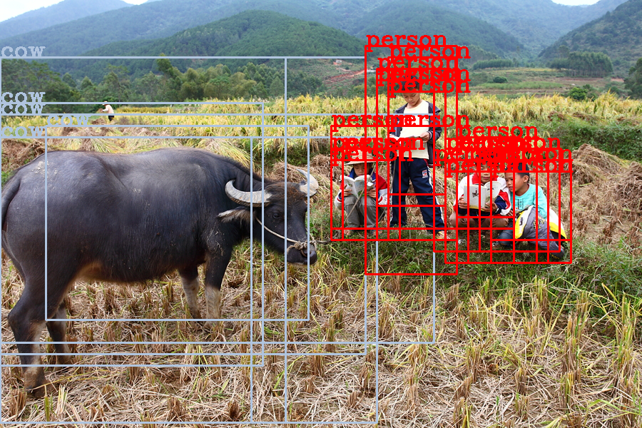
根据类别编号得到该类的边框回归梯度
对回归梯度进行规整化
对预测的边框进行修正
向相应的类里面添加信息【乘 C.rpn_stride,边框的预测都是在特征图上进行的要将其映射到规整后的原图上】1
2
3
4
5
6
7
8
9
10
11
12
13
14
15
16try:
# obtain privous position's bbox's regrient
(tx, ty, tw, th) = P_regr[0, ii, 4*cls_num:4*(cls_num+1)]
# waiting test
tx /= C.classifier_regr_std[0]
ty /= C.classifier_regr_std[1]
tw /= C.classifier_regr_std[2]
th /= C.classifier_regr_std[3]
# fix box with regreient
x, y, w, h = rpn_to_boxes.apply_regr(x, y, w, h, tx, ty, tw, th)
except:
pass
# cordinates of current's box on real img
bboxes[cls_name].append([C.rpn_stride*x, C.rpn_stride*y, C.rpn_stride*(x+w), C.rpn_stride*(y+h)])
# coresspoding posbility
probs[cls_name].append(np.max(P_cls[0, ii, :]))
这样修正过的框可以画在图上: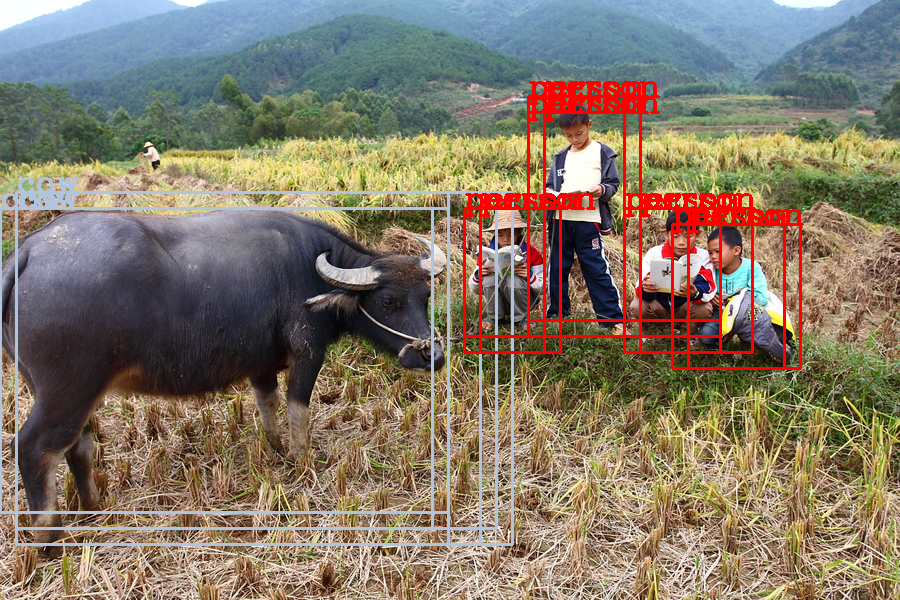
遍历bboxes里的类,取出某一类的bbox,合并一些重合度较高的选框
No Max Supression1
2
3
4
5
6
7# for all classes in current boxes
for key in bboxes:
# bboxes's cordinates
bbox = np.array(bboxes[key])
# apply NMX to merge some overlapping boxes
new_boxes, new_probs = rpn_to_boxes.non_max_suppression_fast(bbox, np.array(probs[key]), overlap_thresh=0.5)
最终的图: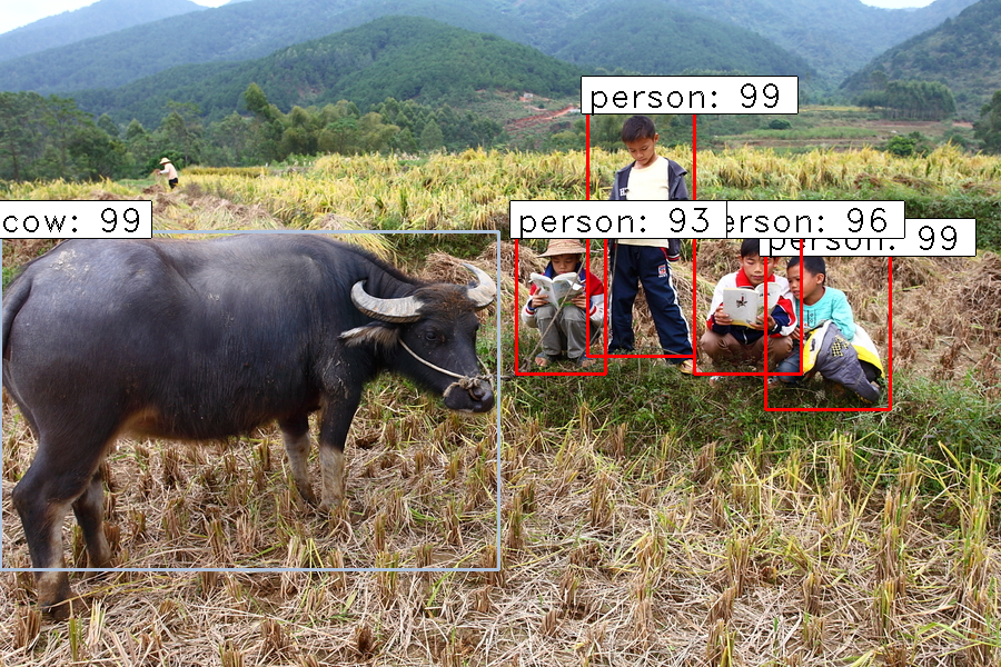
result
Small img, only 8k
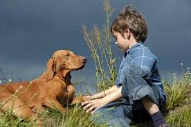
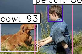
Overlapping img
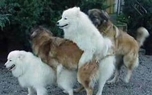
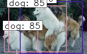
Crowed People

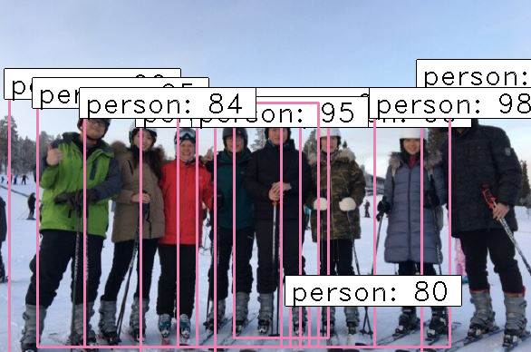
cow and people
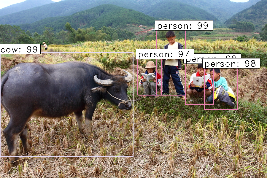
car and plane


Street img

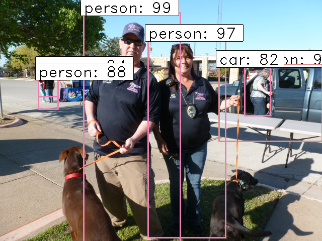
Lots Dogs
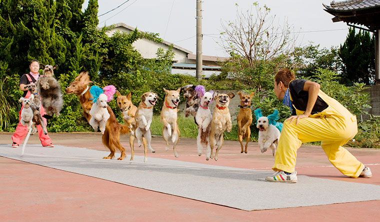
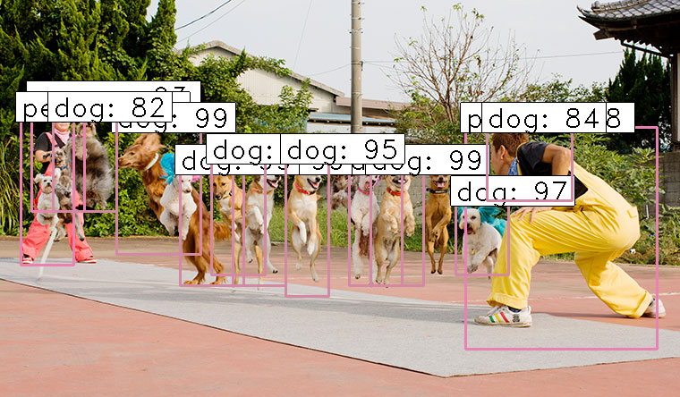
Overlapping car and people
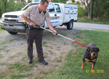
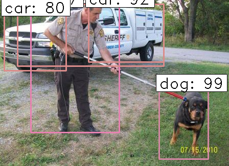
直观看的话效果还不错,但是一些重叠的物体框会出现反复,或者取不到。而且分类有一点过拟合。
【03/08/2018】
evaluation
mAP
mAP是目标算法中衡量算法的精确度的指标,涉及两个概念:查准率Precision、查全率Recall。对于object detection任务,每一个object都可以计算出其Precision和Recall,多次计算/试验,每个类都 可以得到一条P-R曲线,曲线下的面积就是AP的值,这个mean的意思是对每个类的AP再求平均,得到的就是mAP的值,mAP的大小一定在[0,1]区间。
AP:Precision对Recall积分,可通过改变正负样本阈值求得矩形面积,进而求积分得到,也可以通过sklearn.metrics.average_precision_score函数直接得到。
传入预测值和真实值和resize比例,得到可以传入sklearn.metrics.average_precision_score函数的值,即:真实值和预测概率
首先搭建rpn和分类器网络,按照之前的train部分来就可以了
这里注意分类网络的输入换成测试图片的feature map1
2
3
4
5
6
7
8
9
10num_features = 1024
input_shape_img = (None, None, 3)
input_shape_features = (None, None, num_features)
img_input = Input(shape=input_shape_img)
roi_input = Input(shape=(C.num_rois, 4))
feature_map_input = Input(shape=input_shape_features)
classifier = nn.classifier(feature_map_input, roi_input, C.num_rois, nb_classes=len(class_mapping), trainable=True)
然后载入需要测试的模型权重
按照VOC的数据集标注,把测试集分出来:1
2
3
4
5
6
7
8train_imgs = []
test_imgs = []
for each in all_imgs:
if each['imageset'] == 'trainval':
train_imgs.append(each)
if each['imageset'] == 'test':
test_imgs.append(each)
按照之前的预测方法,求出图片的预测框坐标以及对应的分类名字,然后把这些信息放入对应的字典里面,与xml解析的文件一样的格式:1
2
3
4for jk in range(new_boxes.shape[0]):
(x1, y1, x2, y2) = new_boxes[jk, :]
det = {'x1': x1, 'x2': x2, 'y1': y1, 'y2': y2, 'class': key, 'prob': new_probs[jk]}
all_dets.append(det)
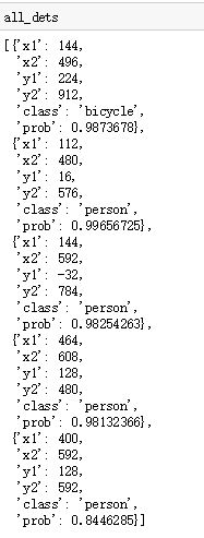
然后读取标注的框的真实数值: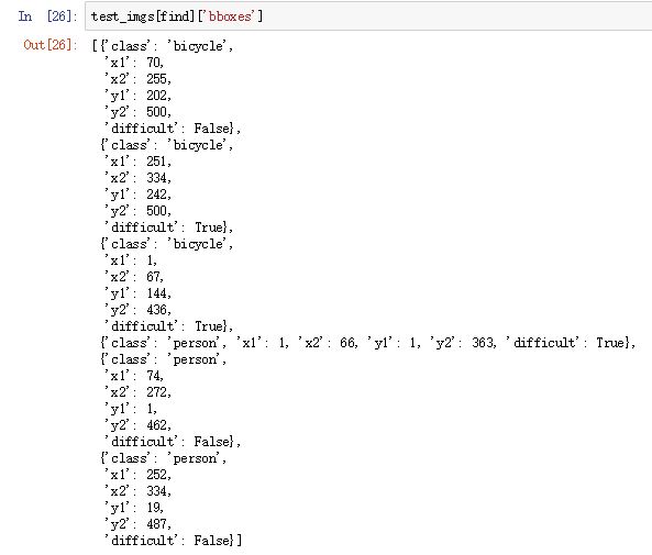
遍历真实信息里面的每一个狂,将bbox_matched这个属性标注为FALSE,之后如果预测框和标注框对应上的话,这个属性就会被设置为True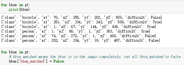
获取预测框里面的分类对应概率,并且按照概率从大到小得到idx位置: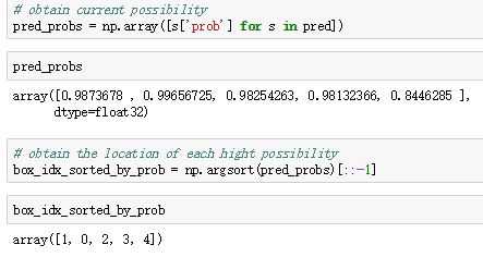
按照概率大小,对每一个对应的预测框,对比每一个标注的框,如果预测的类与当前标注框的类相同并且没有被匹配过,计算两个框的iou,如果大于0.5的话就表明预测框匹配当前标注框,保存预测概率以及对应的是否匹配:
1 | # process each bbox with hightest prob |
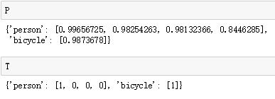
遍历每一个标注框,如果没有被匹配到并且diffcult属性不是true的话,说明这个框漏检了,在之前保存的概率以及对应是否有概率里面加入物体1以及对应概率01
2
3
4
5
6
7
8
9
10# adding missing object compared to orignal image
for gt_box in gt:
if not gt_box['bbox_matched'] and not gt_box['difficult']:
if gt_box['class'] not in P:
P[gt_box['class']] = []
T[gt_box['class']] = []
# T = 1 means there are object, P = 0 means we did't detected that
T[gt_box['class']].append(1)
P[gt_box['class']].append(0)
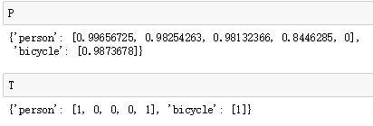
把当前信息存入到总的一个词典里面,就可以使用average_precision_score这个sklearn里面的函数计算ap了。与此同时,保存得到的结果并且显示总的map: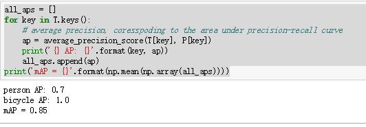
【06~10/08/2018】
adjust
将计算ap的函数包装好:
jupyter notebook
Project1 all: 9 models:
ALL_2 NO THRESHOLD OTHER WITH THRESHOLD MOST 0.8
| Classes | ALL_1 | ALL_2 | ALL_3 | ALL_4 | ALL_5 | ALL_6 | ALL_7 | ALL_8 | ALL_9 |
|---|---|---|---|---|---|---|---|---|---|
| motorbike | 0.2305 | 0.2412 | 0.2132 | 0.2220 | 0.2889 | 0.2528 | 0.2204 | 0.2644 | 0.2336 |
| person | 0.6489 | 0.6735 | 0.7107 | 0.6652 | 0.7120 | 0.7041 | 0.7238 | 0.7003 | 0.7201 |
| car | 0.1697 | 0.1563 | 0.2032 | 0.2105 | 0.2308 | 0.2221 | 0.2436 | 0.2053 | 0.2080 |
| aeroplane | 0.7968 | 0.7062 | 0.7941 | 0.6412 | 0.7871 | 0.7331 | 0.7648 | 0.7659 | 0.6902 |
| bottle | 0.2213 | 0.2428 | 0.2261 | 0.1943 | 0.2570 | 0.2437 | 0.2899 | 0.1442 | 0.2265 |
| sheep | 0.6162 | 0.5702 | 0.6876 | 0.6295 | 0.6364 | 0.5710 | 0.6536 | 0.6349 | 0.6455 |
| tvmonitor | 0.1582 | 0.1601 | 0.2231 | 0.1748 | 0.1551 | 0.1603 | 0.1317 | 0.1584 | 0.1678 |
| boat | 0.3842 | 0.2621 | 0.2261 | 0.1943 | 0.3499 | 0.2437 | 0.2057 | 0.2748 | 0.3509 |
| chair | 0.2811 | 0.0563 | 0.0891 | 0.0621 | 0.1353 | 0.0865 | 0.0907 | 0.0854 | 0.1282 |
| bicycle | 0.1464 | 0.1224 | 0.1346 | 0.1781 | 0.1406 | 0.1448 | 0.1810 | 0.1071 | 0.1673 |
| cat | 0.8901 | 0.8565 | 0.9103 | 0.8417 | 0.8289 | 0.8274 | 0.7572 | 0.9143 | 0.8118 |
| pottedplant | 0.2075 | 0.0926 | 0.1790 | 0.0532 | 0.1517 | 0.1150 | 0.1080 | 0.1022 | 0.0939 |
| horse | 0.1185 | 0.0588 | 0.0726 | 0.0489 | 0.0696 | 0.0695 | 0.0637 | 0.0651 | 0.0640 |
| sofa | 0.2797 | 0.2309 | 0.2852 | 0.2966 | 0.3855 | 0.4817 | 0.3659 | 0.3132 | 0.3090 |
| dog | 0.5359 | 0.5077 | 0.5578 | 0.4413 | 0.4832 | 0.5793 | 0.5687 | 0.4910 | 0.4598 |
| cow | 0.7582 | 0.6229 | 0.7295 | 0.5420 | 0.5379 | 0.5312 | 0.5147 | 0.5706 | 0.6503 |
| diningtable | 0.3979 | 0.2734 | 0.3739 | 0.2963 | 0.4715 | 0.4987 | 0.3895 | 0.4983 | 0.4666 |
| bus | 0.6203 | 0.5572 | 0.6468 | 0.6032 | 0.6320 | 0.6096 | 0.7169 | 0.5938 | 0.5485 |
| bird | 0.6164 | 0.6662 | 0.5692 | 0.5751 | 0.5407 | 0.4125 | 0.4925 | 0.4347 | 0.5208 |
| train | 0.8655 | 0.6916 | 0.7141 | 0.7166 | 0.7643 | 0.8107 | 0.7100 | 0.7194 | 0.6263 |
| mAP | 0.4472 | 0.3874 | 0.4341 | 0.3859 | 0.4279 | 0.4141 | 0.4096 | 0.4022 | 0.4045 |
Project1 epoch_lenght=1000, epoch:1041 : 7 models:
ALL WITH THRESHOLD MOST 0.51
| Classes | ALL_1 | ALL_2 | ALL_3 | ALL_4 | ALL_5 | ALL_6 | ALL_7 |
|---|---|---|---|---|---|---|---|
| motorbike | 0.2433 | 0.2128 | 0.2232 | 0.2262 | 0.2286 | 0.2393 | 0.2279 |
| person | 0.6560 | 0.6537 | 0.6742 | 0.6952 | 0.6852 | 0.6719 | 0.6636 |
| car | 0.1562 | 0.1905 | 0.1479 | 0.2024 | 0.2010 | 0.1379 | 0.1583 |
| aeroplane | 0.7359 | 0.6837 | 0.6729 | 0.6687 | 0.6957 | 0.7339 | 0.6391 |
| bottle | 0.1913 | 0.1937 | 0.2635 | 0.1843 | 0.2570 | 0.1632 | 0.1863 |
| sheep | 0.5429 | 0.5579 | 0.6219 | 0.5355 | 0.5881 | 0.5441 | 0.5824 |
| tvmonitor | 0.1295 | 0.1601 | 0.1368 | 0.1407 | 0.1147 | 0.1349 | 0.1154 |
| boat | 0.1913 | 0.2880 | 0.2635 | 0.3433 | 0.3335 | 0.3422 | 0.3069 |
| chair | 0.0587 | 0.0657 | 0.0342 | 0.0680 | 0.0695 | 0.0752 | 0.0760 |
| bicycle | 0.1013 | 0.1485 | 0.1225 | 0.1871 | 0.1685 | 0.1037 | 0.1490 |
| cat | 0.8737 | 0.8557 | 0.8007 | 0.7982 | 0.8045 | 0.8067 | 0.7732 |
| pottedplant | 0.0694 | 0.1059 | 0.0748 | 0.0878 | 0.0893 | 0.0690 | 0.0865 |
| horse | 0.0556 | 0.0561 | 0.0581 | 0.0770 | 0.0575 | 0.0539 | 0.0522 |
| sofa | 0.2177 | 0.2917 | 0.1699 | 0.1940 | 0.3177 | 0.1863 | 0.1857 |
| dog | 0.6269 | 0.4989 | 0.5015 | 0.5333 | 0.4914 | 0.5572 | 0.4747 |
| cow | 0.5216 | 0.6229 | 0.5283 | 0.6426 | 0.4358 | 0.4227 | 0.4589 |
| diningtable | 0.3076 | 0.3889 | 0.3283 | 0.2404 | 0.4219 | 0.4153 | 0.2627 |
| bus | 0.5865 | 0.5222 | 0.6312 | 0.5853 | 0.5042 | 0.4882 | 0.5576 |
| bird | 0.5339 | 0.5039 | 0.5150 | 0.5152 | 0.5838 | 0.3890 | 0.4680 |
| train | 0.4994 | 0.6541 | 0.6702 | 0.6920 | 0.5959 | 0.5893 | 0.6861 |
| mAP | 0.3699 | 0.3765 | 0.3748 | 0.3814 | 0.3786 | 0.3562 | 0.3555 |
在测试集上的结果不是很好,不同class的ap差距较大,可能是由于训练时候不平均或者训练集太小的原因
尝试加入VOC2007的数据进训练集当中,观察结果。
解析VOC2007的过程中遇到了OpenCV读取不了图片的BUG。
(已修复)
VOC2012的数据莫名没有了,因为之前测试过的原因,一直以为是VOC2007的数据解析有问题,大概是Irius的文件上限时间到了自动清除了数据。
20个类当中的AP差距过大,其实数据集是不平衡的,有的类只有大概1000个样本,但是人这个样本就有2W多,而且之前的训练过程中每次图片都是在训练集中随机选的,所以尝试修改了流程,当所有训练集中的数据都被读取训练过以后再打乱训练集,与此同时配合class_balance的功能使用。
实际上使用的时候class balance效果不是很好,后面没有开启。
用了一个较大的学习率尝试训练没有载入imagenet预训练权重的版本。
交叉法
【13/08/2018】
soft-NMS
传统的非最大抑制算法首先在被检测图片中产生一系列的检测框B以及对应的分数S。当选中最大分数的检测框M,它被从集合B中移出并放入最终检测结果集合D。于此同时,集合B中任何与检测框M的重叠部分大于重叠阈值Nt的检测框也将随之移除。非最大抑制算法中的最大问题就是它将相邻检测框的分数均强制归零。在这种情况下,如果一个真实物体在重叠区域出现,则将导致对该物体的检测失败并降低了算法的平均检测率(average precision, AP)。
换一种思路,如果我们只是通过一个基于与M重叠程度相关的函数来降低相邻检测框的分数而非彻底剔除。虽然分数被降低,但相邻的检测框仍在物体检测的序列中。图二中的实例可以说明这个问题。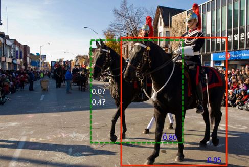
针对NMS存在的这个问题,我们提出了一种新的Soft-NMS算法(图三),它只需改动一行代码即可有效改进传统贪心NMS算法。在该算法中,我们基于重叠部分的大小为相邻检测框设置一个衰减函数而非彻底将其分数置为零。简单来讲,如果一个检测框与M有大部分重叠,它会有很低的分数;而如果检测框与M只有小部分重叠,那么它的原有检测分数不会受太大影响。在标准数据集PASCAL VOC 和 MS-COCO等标准数据集上,Soft-NMS对现有物体检测算法在多个重叠物体检测的平均准确率有显著的提升。同时,Soft-NMS不需要额外的训练且易于实现,因此,它很容易被集成到当前的物体检测流程中。
伪代码: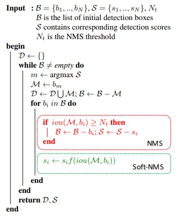
公式:
NMS
$$ s_{i}=\left{
\begin{aligned}
s_{i}, \ \ \ \ iou(M,b_{i}) < N_{t} \
0, \ \ \ \ iou(M,b_{i}) \geq N_{t}
\end{aligned}
\right.
$$
SOFT NMS
$$ s_{i}=\left{
\begin{aligned}
s_{i}, \ \ \ \ iou(M,b_{i}) < N_{t} \
1-iou(M,b_{i}), \ \ \ \ iou(M,b_{i}) \geq N_{t}
\end{aligned}
\right.
$$
当相邻检测框与M的重叠度超过重叠阈值Nt后,检测框的检测分数呈线性衰减。在这种情况下,与M相邻很近的检测框衰减程度很大,而远离M的检测框并不受影响。
但是,上述分数重置函数并不是一个连续函数,在重叠程度超过重叠阈值Nt时,该分数重置函数产生突变,从而可能导致检测结果序列产生大的变动,因此我们更希望找到一个连续的分数重置函数。它对没有重叠的检测框的原有检测分数不产生衰减,同时对高度重叠的检测框产生大的衰减。综合考虑这些因素,我们进一步对soft-NMS中的分数重置函数进行了改进:
Gaussian penalty: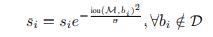
根据这个伪代码以及公式,实现代码:1
2
3
4
5
6
7
8
9
10
11
12
13
14
15
16
17
18
19
20
21
22
23
24
25
26
27
28
29
30
31
32
33
34
35
36
37
38
39
40
41
42
43
44
45
46
47
48
49
50
51
52
53
54
55
56
57
58
59
60
61
62
63
64
65
66
67
68
69
70
71
72
73
74
75
76
77
78
79
80
81
82
83
84
85
86
87
88
89
90
91
92
93
94
95
96
97
98
99
100
101
102
103
104
105
106
107
108
109
110
111
112
113
114
115
116
117
118""" NMS , delete overlapping box
@param boxes: (n,4) box and coresspoding cordinates
@param probs: (n,) box adn coresspding possibility
@param overlap_thresh: treshold of delet box overlapping
@param max_boxes: maximum keeping number of boxes
@param method: 1 for linear soft NMS, 2 for gaussian soft NMS
@param sigma: parameter of gaussian soft NMS
prob_thresh: threshold of probs after soft NMS
@return: boxes: boxes cordinates(x1,y1,x2,y2)
@return: probs: coresspoding possibility
"""
def soft_nms(boxes, probs, overlap_thresh=0.9, max_boxes=300, method = 1, sigma=0.5, prob_thresh=0.49):
# number of input boxes
N = boxes.shape[0]
# if the bounding boxes integers, convert them to floats --
# this is important since we'll be doing a bunch of divisions
if boxes.dtype.kind == "i":
boxes = boxes.astype("float")
# iterate all boxes
for i in range(N):
# obtain current boxes' cordinates and probs
maxscore = probs[i]
maxpos = i
tx1 = boxes[i,0]
ty1 = boxes[i,1]
tx2 = boxes[i,2]
ty2 = boxes[i,3]
ts = probs[i]
pos = i + 1
# get max box
while pos < N:
if maxscore < probs[pos]:
maxscore = probs[pos]
maxpos = pos
pos = pos + 1
# add max box as a detection
boxes[i,0] = boxes[maxpos,0]
boxes[i,1] = boxes[maxpos,1]
boxes[i,2] = boxes[maxpos,2]
boxes[i,3] = boxes[maxpos,3]
probs[i] = probs[maxpos]
# swap ith box with position of max box
boxes[maxpos,0] = tx1
boxes[maxpos,1] = ty1
boxes[maxpos,2] = tx2
boxes[maxpos,3] = ty2
probs[maxpos] = ts
# cordinates of max box
tx1 = boxes[i,0]
ty1 = boxes[i,1]
tx2 = boxes[i,2]
ty2 = boxes[i,3]
ts = probs[i]
pos = i + 1
# NMS iterations, note that N changes if detection boxes fall below threshold
while pos < N:
x1 = boxes[pos, 0]
y1 = boxes[pos, 1]
x2 = boxes[pos, 2]
y2 = boxes[pos, 3]
s = probs[pos]
# calculate the areas, +1 for robatness
area = (x2 - x1 + 1) * (y2 - y1 + 1)
iw = (min(tx2, x2) - max(tx1, x1) + 1)
# # confirm left top cordinates less than top right
if iw > 0:
ih = (min(ty2, y2) - max(ty1, y1) + 1)
# confirm left top cordinates less than top right
if ih > 0:
# find the union
ua = float((tx2 - tx1 + 1) * (ty2 - ty1 + 1) + area - iw * ih)
#iou between max box and detection box
ov = iw * ih / ua
if method == 1: # linear
if ov > overlap_thresh:
weight = 1 - ov
else:
weight = 1
elif method == 2: # gaussian
weight = np.exp(-(ov * ov)/sigma)
else: # original NMS
if ov > overlap_thresh:
weight = 0
else:
weight = 1
# obtain adjusted probs
probs[pos] = weight*probs[pos]
# if box score falls below threshold, discard the box by swapping with last box
# update N
if probs[pos] < prob_thresh:
boxes[pos,0] = boxes[N-1, 0]
boxes[pos,1] = boxes[N-1, 1]
boxes[pos,2] = boxes[N-1, 2]
boxes[pos,3] = boxes[N-1, 3]
probs[pos] = probs[N-1]
N = N - 1
pos = pos - 1
pos = pos + 1
# keep is the idx of current keeping objects, front ith objectes
keep = [i for i in range(N)]
return boxes[keep], probs[keep]
